5  Emergence

posts/050-emergence.qmd

Compiled: 2026-02-28 09:49:34.646941200

posts/050-emergence.qmd

5.1 Introduction

posts/050-files/introduction.qmd

This introduction lays out the conditional probability notation and concepts we need and then introduces two models, the P2P and DMC that we go on to consider in more detail.

5.1.1 Conditional Probability

We work in discrete time \(t=0,1,2\) on a probability space \((\Omega,\mathscr F,\mathsf P)\) with a filtration \[ \mathscr F_0\subset \mathscr F_1\subset \mathscr F_2=\mathscr F. \] Here \(\mathscr F_t\) represents the information available at time \(t\). Let \(X\) denote the ultimate loss of a policy (or portfolio), which is revealed by time \(2\). Thus \(X\) is \(\mathscr F_2\)-measurable. \(\mathscr F_0=\set{\emptyset, \Omega}\) contains no information about future losses.

The point of a multi-period model is simple: at time \(1\) the insurer knows more than at time \(0\), and the value assigned to \(X\) at time \(1\) depends on that new information, but further uncertainty remains. We represent the time-1 information by a state variable \(S\).

For simplicity, we assume that \(S\) has a finite range, \[ S\in \set{1,\dots,k}, \] and assume it encodes all information revealed at \(t=1\) \[ \mathscr F_1=\sigma(S). \] This assumption says that time-1 information is exactly the observed state. In particular, a random variable \(Y\) is \(\mathscr F_1\)-measurable, meaning its value is known at \(t=1\), if and only if there is a function \(y\) such that \(Y=y(S)\). In a finite-state model, \(\mathscr F_1\)-measurable objects are lookup tables indexed by the state. In our application, \(S\) might encode information about reported claims used to set case reserves, as well as macroeconomic and environmental information used in bulk reserving.

Actuaries usually meet conditioning as a number, \(\mathsf E[X\mid S=s]\). In a multi-period model, conditioning appears as a function of the realized state. We write conditional expectation as \[ \mathsf P_S(X):=\mathsf P(X\mid \mathscr F_1), \] meaning the best estimate (mean) of \(X\) given state \(S\). Since \(\mathscr F_1=\sigma(S)\), the random variable \(\mathsf P_S(X)\) is \(\mathscr F_1\)-measurable and therefore a function of \(S\). Write \[ \mathsf P_S(X)=r(S) \] which means \[ r(s):=\mathsf P(X\mid S=s). \] (As a random variable, \(r(S)(\omega)=r(S(\omega))\).) The function \(r\) is the best estimate reserve evaluated at time \(1\). The type of reserve depends on the definition of \(X\): it could be case if \(X\) pertains to a single claim or case plus IBNR if \(X\) is modeling reported and unreported claims on a portfolio. Once the state \(S\) is observed, the reserve is the number \(r(S)\). In a finite-state model, the entire conditional expectation \(\mathsf P_S(X)\) is nothing more than the \(k\) values \({r(1),\dots,r(k)}\) attached to the \(k\) states.

5.1.2 Disintegration or Decomposition of Probabilities

We assume a regular conditional probability exists so that conditioning corresponds to a two-stage decomposition or “disintegration” of \(\mathsf P\). The state \(S\) has a marginal law, denoted \(\mathsf P^S\), defined by \[ \mathsf P^S(A) = \mathsf P(S^{-1}(A)) = \mathsf P\set{\omega \middle S(\omega) = k} \] for \(A \subset \set{1,\dots,k}\). In addition, there is a conditional law given the state, denoted \(\mathsf P_S\). Informally, to arrive at at \(t=2\) outcome, we first draw \(S\sim \mathsf P^S\), and then, given \(S=s\), draw the remaining uncertainty according to \(\mathsf P_s\). This is the multi-period version of “state then development.”

With \(S\in\set{1,\dots,k}\), the law \(\mathsf P\) decomposes (disintegrates) into a mixture of the conditional laws \(\set{\mathsf P_s}_{s=1}^k\) with mixing weights given by the state probabilities \(\mathsf P^S(s)=\mathsf P\set{S=s}\). Concretely, for any event \(A\in\mathscr F\), \[ \mathsf P(A)=\sum_{s=1}^k \mathsf P^S(s)\,\mathsf P_s(A). \] This identity is the easiest way to remember what “conditioning on \(S\)” means: \(\mathsf P_s(\cdot)\) is the state-\(s\) world, and \(\mathsf P^S\) averages those worlds using the probability of each state.

Applying the same mixture idea to a random variable \(X\) gives \[ \mathsf P(X)=\sum_{s=1}^k \mathsf P^S(s)\,\mathsf P_s(X). \] Now define the time-1 best estimate reserve by \[ r(s):=\mathsf P_s(X),\qquad \mathsf P_S(X)=r(S). \] Then \[ \mathsf P(X)=\sum_{s=1}^k \mathsf P^S(s)\,r(s)=\mathsf P^S\big(r(S)\big). \] Thus the unconditional mean loss is the state-probability-weighted average of the statewise best estimate reserves.

Remark 5.1. \(\mathsf P_s(\cdot)\) is the regular conditional probability \(\mathsf P(\cdot\mid S=s)\), viewed as a probability measure indexed by the realized state (Kallenberg 2021).

Remark 5.2 (Disintegration and conditional probability). Integration builds a joint law from pieces. Start with a marginal law on states, \(\mathsf P^S\) on \({1,\dots,k}\), and a family of conditional laws \({\mathsf P_s}_{s=1}^k\) on \((\Omega,\mathcal F)\). These pieces define a probability measure \(\mathsf P\) on the product space \({1,\dots,k}\times\Omega\) by \[ \mathsf P({s}\times A):=\mathsf P^S(S=s),\mathsf P_s(A),\qquad A\in\mathcal F. \] Extending by additivity gives a joint law on the product. In this direction, the joint measure is a mixture of the kernels \(\mathsf P_s\).

Disintegration recovers the pieces from the joint law. Now, go the other way: start with a single probability measure \(\mathsf P\) on \({1,\dots,k}\times\Omega\) and define the state variable \(S(s,\omega)=s\). Then \(\mathsf P\) determines a marginal law \(\mathsf P^S\) for \(S\), and, for each \(s\) with \(\mathsf P^S(S=s)>0\), a conditional law \(\mathsf P_s\) on \((\Omega,\mathcal F)\) such that \[ \mathsf P({s}\times A)=\mathsf P^S(S=s),\mathsf P_s(A). \] The family \(s\mapsto \mathsf P_s\) is exactly a regular conditional probability for the second coordinate given \(S=s\).

In this finite-state setting, disintegration solves for the conditional laws: \[ \mathsf P_s(A)=\mathsf P(A\mid S=s). \] The same idea works in general state spaces, but existence and uniqueness become technical, which is why we state it as an assumption when needed.

5.1.3 From Single-Period to Multi-Period Pricing

The actuarial value of cash flows take expectations using \(\mathsf P\) and so multi-period bookkeeping collapses to a mixture across states. The tower property of conditional expectations means there is no difference between single- and multi-period expectations. Pricing replaces \(\mathsf P(\cdot)\) with a one-period pricing functional \(g(\cdot)\) and asks a basic question: If we can price one-period uncertainty, how can we price a multi-period liability?

There are many answers in the literature, and we focus on two: broadly an accident year ultimate view, and a calendar year steady-state view. They agree under \(\mathsf P\), but typically differ under \(g\).

We keep same notation: the \(t=0,1,2\) timeline and write \(S\) for the time-1 state with \(\mathscr F_1=\sigma(S)\). Think of \(S\) as the end-of-calendar-year information used to set reserves, and think of \(X\) as the ultimate loss. For simplicity we assume no discount. Ch REF1 treated discount without emergence and Ch REF2 combines discount and emergence to create the full picture.

The first construction is called P2P or policy to buy a policy pricing, also known as iterative pricing in the literature. It prices in two stages, mirroring the decomposition of \(\mathsf P\) as emerged state and then development. At time \(1\), after observing \(S\), price the remaining one-period uncertainty in \(X\) under the conditional model. This produces a time-1 value \[ V_1 := g^{\mathsf P_S}(X), \] a state-contingent quantity, and hence a function of \(S\).

Then, from time \(0\), price that time-1 random value across states: \[ V_0^{\mathrm{P2P}} := g^{\mathsf P^S}(V_1)=g^{\mathsf P^S}\!\big(g^{\mathsf P_S}(X)\big). \]

The time-1 step, \(g^{\mathsf P_S}(X)\), is an IFRS-style “best estimate plus risk adjustment” conditional on the information available at \(t=1\). The time-0 step prices the randomness of that risk-adjusted reserve across states. This is the source of “risk load on risk load.” Even if \(g\) is calibrated so that \(g^{\mathsf P_S}(X)\) adds a risk adjustment to the conditional best estimate in each state, the second application of \(g\) adds a further adjustment for variation in that reserve across states. We assume that \(g\) is constant, so there is no market cycle shift. Allow \(g\) to evolve over time is an obvious idea, but a massive increase in complexity and is left for future research.

P2P a natural construction when the economic story is genuinely sequential: the contract is repriced, or capital is rolled forward, as information arrives. It is also a natural construction if one wants a time-consistent valuation rule, in the sense that values are built by composing one-period valuations along the filtration.

The second construction, DMC or decoupled marginal cost, takes a different view. Instead of iterating prices along a single accident year, it builds a one-period portfolio that represents a steady-state calendar year of development and prices its one-period risk using \(g\).

The calendar-year viewpoint is familiar to actuaries: in calendar year \(t=0\to1\) the firm experiences one year of development on many accident years. DMC formalizes that idea by forming a one-calendar-period development slice from each accident year, pooling them into a single one-year aggregate, pricing that aggregate with \(g\), and then allocating the priced margin back to the accident years using the natural allocation. It is called decoupled because prior accident years are more mutually independent that sequential development from the same accident year. The base DMC model assumes prior accident years are all independent, a standard modeling choice (Mack 1993).

DMC has a conceptual and practical simplicity. \(g\) is used once, on a one-period calendar-year aggregate. We are only projecting forward one-year, regardless of the number of historical accident years. The resulting risk adjustment is naturally interpreted as a margin recognized over the calendar year. Any remaining margin that is not recognized immediately is deferred by construction, rather than arising from a second application of \(g\).

This makes DMC a natural construction when the operational unit is the calendar year, and when the accounting story earns one year of risk adjustment as one year of development occurs. It ties well with IFRS 17 requirements.

To conclude the introduction:

• P2P is accident-year native. It follows a single policy (or accident year cohort) as information arrives and revalues the remaining liability at each step.
• DMC is calendar-year native. It prices the risk of the next calendar year’s development, as a pooled one-period problem, and then attributes the result back to accident years.

Under \(\mathsf P\), these perspectives are just alternative descriptions of the same expectation. Under \(g\), they generally lead to different values because the mixture across states that makes conditioning easy under \(\mathsf P\) does not commute with nonlinear pricing. The next sections make that difference concrete. We start by introducing an example and then analyzing its P2P and DMC pricing.

5.2 Two Pricing Models for Bernoulli Risks with Simple Information

posts/050-files/two-pricing-models.qmd

Multi-period pricing looks deceptively close to single-period pricing: a loss either happens or it does not, and a one-period pricing rule assigns a premium. The complication is time and information. Real liabilities do not arrive fully formed. Estimates, reports, and model updates arrive in stages, and those stages change the best estimate of the remaining liability. Accounting rules mean adverse development cannot be wished away, and recognizing it has an economic cost.

This section studies a deliberately stylized framework for a two-period emergence with a Bernoulli risk driven by a latent uniform variable. If we can’t solve the problem in this simple world, we’ll never succeed in the real world! We then present two models: P2P and DMC. Both use SRMs to price risk. The P2P model prices a multi-period risk by composing the same one-period pricing rule across time. It can be interpreted as the price for a replicating portfolio consisting of a “policy to buy a policy”, hence the name. The DMC decoupled marginal cost model sets up a calendar year portfolio with a new accident year and a generic prior year’s reserves, and prices it from the top-down using the SRM.

Both models are simple enough to analyze by hand, but still capture two features that matter in practice.

1. Information about the latent variable arrives at an interim date and changes the conditional distribution of what remains.
2. The pricing rules react to that interim update in a way that depends on risk appetite, as encoded by the underlying SRM.

We see pricing depends both on the SRM and the way information emerges. The key findings are that the “best” interim information depends on risk appetite as encoded in the pricing rule, and that not all appetites value interim information in the same way. Moreover, P2P and DMC may differ in their view of the economic cost of multi-period emergence. In this model, “best” means the interim disclosure that minimizes the two-period price. We analyze when the two-period price is uniformly lower or higher than the single-period price. For P2P we are led to consider whether the SRM is sub- or super-multiplicative, as described in sec-040-100.

These considerations matter. Insurance lines differ in emergence patterns. Property catastrophe risk tends to emerge quickly; casualty and liability risk often emerges slowly, with information arriving over extended periods. This section illustrates how a pricing rules value interim information, and why that valuation differs between risk appetites.

The next subsections describe the framework components.

5.2.1 Discount

We assume the discount rate is zero. The model we are describing reflects loss emergence, not loss discounting. Discount is relatively easy to incorporate once emergence has been addressed. This chapter parallels sec-bullets, which considered discount without modeling emergence.

5.2.2 The Risk

We price a Bernoulli random variable defined as follows. Let \(U\) be uniform on \([0,1]\). Fix a loss probability \(s\in(0,1)\) and define the Bernoulli loss as the indicator function \[ X=\set{U<s}. \] Thus \(X\) takes values in \(\{0,1\}\) with \(\mathsf P(X=1)=s\).

5.2.3 The One-Period Pricing Rule

Fix SRM defined by a concave distortion function \(g\). In one period, the price of the Bernoulli-\(s\) loss is \[ g(X) = g(s). \] We use \(g\) as notation for both the distortion and the induced one-period pricing rule on Bernoulli indicators.

5.2.4 Interim Information

Information flow is extremely complicated. The framework we introduce here restricts information to what we call simple information: a single yes/no message. At time \(t=1\), we receive a message determined by a threshold \(\omega_I\in(0,1)\):

• message A: \(U\le \omega_I\),
• message B: \(U> \omega_I\).

At this point, we avoid \(\sigma\)-algebras and think only in terms of the revealed message. The message partitions the world into two states, and in each state the remaining liability \(X\) has a conditional distribution. We write “\(X\) given the message” as \(X_I\).

5.2.5 The Meaning of “\(X\) Given the Message”

Because \(X=\set{U<s}\) is a function of \(U\), conditioning on the message just means restricting \(U\) to the relevant interval and re-evaluating the chances \(U<s\). There are three cases.

Case 1: \(\omega_I<s\).

• If message A occurs (\(U\le\omega_I\)), then \(U<s\) holds for sure, so \[ X_I = X \mid (U\le\omega_I) = 1 \quad\text{(certain loss)}. \]

• If message B occurs (\(U>\omega_I\)), then \(U\) is uniform on \((\omega_I,1]\). The event \(\set{U<s}\) becomes a Bernoulli event with reduced probability \[ s_I=\mathsf P(U<s\mid U>\omega_I)=\frac{s-\omega_I}{1-\omega_I}, \] so we can represent the conditional loss as \[ X_I = X \mid (U>\omega_I)\ \sim\ \text{Bernoulli}(s_I). \]

Case 2: \(\omega_I>s\).

• If message B occurs (\(U>\omega_I\)), then \(U<s\) is impossible, so \[ X_I = X \mid (U>\omega_I) = 0 \quad\text{(certain no-loss)}. \]

• If message A occurs (\(U\le\omega_I\)), then \(U\) is uniform on \([0,\omega]\). The event \(\set{U<s}\) becomes a Bernoulli event with increased probability \[ s_I = \mathsf P(U<s\mid U\le\omega_I)=\frac{s}{\omega_I}, \] so \[ X_I = X \mid (U\le\omega_I)\ \sim\ \text{Bernoulli}(s_I). \]

Case 3: \(\omega_I=s\).

• The message fully reveals the outcome: on \(U\le s\) we have \(X=1\), and on \(U>s\) we have \(X=0\).

Cases 1 and 2 reduce interim disclosure to a clean trade-off.

• In Case 1 we learn either that a loss is certain, or that the remaining loss is less likely.
• In case 2 we learn either that no loss is certain, or that the remaining loss is more likely.

Different risk appetites can value these trade-offs differently. Some place a high premium on ruling out loss, others are more sensitive to confirming loss early, and still others react primarily to how the conditional loss probability shifts. This simple dichotomy foreshadows the results that follow.

5.2.6 Time expense

Define the time expense of the information choice \(\omega_I\) as the difference between a multi-year pricing functional \(g_I\) depending on information \(I\) and one-year price: \[ \tau(\omega_I)=g_I(X) - g(X). \] A positive value indicates information is time expensive and a negative value that it is time cheap. For a given \(g\), we want to know if and when there is a choice of information making pricing time cheap or expensive for all Bernoulli risks.

5.2.7 Simple BTE

Definition 5.1 A distortion \(g\) is simple Bernoulli time expensive (simple BTE) if \(g_I(X)\ge g(X)\) for every Bernoulli \(X=\set{U<s}\), \(s\in(0,1)\), and every choice of simple information \(\omega_I\in(0,1)\). It is simple Bernoulli time cheap (simple BTC) if there exists some choice of simple information so that \(g_I(X)\le g(X)\).

The distortion \(g\) is simple BTC if there is a way to select information \(\omega_I\) so that the \(g_I\) price is less than the one-year price. It is called simple BTC because we are restricting the information to just revealing \(U>\omega_I\) or \(\le \omega_I\). Using this terminology, we can describe the link between time expense and properties of the risk appetite encoded by \(g\).

5.3 The Policy to Buy a Policy (P2P) Model

posts/050-files/p2p-analysis.qmd

5.3.1 Definition

P2P prices over two periods by iterating the same one-period rule. Continue the framework and notation from sec-050-simple.

Step 1. Once the message is known at \(t=1\), the remaining liability from \(t=1\) to \(t=2\) is a one-period Bernoulli (or a constant) in that state. Its time 1 price is therefore:

• in a state where \(X\) is certainly \(1\), the time 1 price is \(1\),
• in a state where \(X\) is certainly \(0\), the time 1 price is \(0\),
• in a state where \(X\) is Bernoulli with adjusted probability \(s_I\), the time 1 price is \(g(s_I)\).

This produces a \(t=1\) value that depends on which message arrived. Call that \(t=1\) random value \(V_1=V_1(\omega)\).

Step 2. At \(t=0\), before the message is known, we price the random value \(V_1\) using the same distortion \(g\).

This yields the two-period P2P price \(g_I(X)\).

For the Bernoulli risk \(X=\set{U<s}\) and information threshold \(\omega_I\in(0,1)\), the P2P price becomes \[ g_I(X)= \begin{cases} g\left(\displaystyle\frac{s-\omega_I}{1-\omega_I} \right)\bigl(1-g(\omega_I)\bigr) + g(\omega_I), & \omega_I < s, \\[1em] g\left(\displaystyle\frac{s}{\omega_I} \right)g(\omega_I), & \omega_I > s. \end{cases} \] This is just “price the time 1 state-values using the time 0 state-prices”. Why? In Case 1 \(V_1\) takes value \(1\) and \(v:=g(s-\omega_I) / g(1-\omega_I))\) with probabilities \(\omega_I\) and \(1-\omega_I\). Since \(1>v\) the SRM prices the first state at \(g(\omega_I)\) and hence the second at \(1-g(\omega_I)\). In Case 2, the outcomes values are \(0\) and \(g(s/\omega_I)\). Now, the second term is larger and picks up weight \(g(1-\omega_I)\) (see REF to how SRMs are computed).

Next, we apply the stochastic framework and one-period pricing rule to explore properties of the P2P price. The Table tbl-states lays out the two states revealed by knowing \(\omega\in(0,\omega_I]\) or \(\omega\in(\omega_I, 1]\). It shows

• the state (conditional) mean,
• the state value \(g(X\mid I)\), which corresponds to the market value of the remaining liability given the interim information,
• the state probability (\(\omega_I\) or \(1-\omega_I\)), the objective probability of the state, and
• the state price as determined by \(g\), the market value price of the state.

For the state price, in case 1 the certain loss is the higher value state and for case 2 it is the possible loss. The lower value state has price given by the complement.

Table 5.1: The two states revealed by \(\omega\in(0,\omega_I]\) or \(\omega\in(\omega_I, 1]\).

State	State Mean	State Value	State Probability	State Price
Case 1: \(\omega_I < s\)
\([0, \omega_I)\)	\(1\)	\(1\)	\(\omega_I\)	\(g(\omega_I)\)
\([\omega_I,1]\)	\(s_I=(s-\omega_I)/(1-\omega_I)\)	\(g(s_I)\)	\(1-\omega_I\)	\(1-g(\omega_I)\)
Case 2: \(\omega_I > s\)
\([0, \omega_I)\)	\(s_I=s/\omega_I\)	\(g(s_I)\)	\(\omega_I\)	\(g(\omega_I)\)
\([\omega_I,1]\)	\(0\)	\(0\)	\(1-\omega_I\)	\(1-g(\omega_I)\)

The first state includes a risk load in both cases, but the state value only includes a risk load in case 2. In both cases \(g_I(X)\) is given by the expectation of the state value with respect to the state price (risk-adjusted) probabilities. The values are \[ g_I(X)= \begin{cases} g\left(\displaystyle\frac{s-\omega_I}{1-\omega_I} \right)(1-g(\omega_I)) + g(\omega_I) & \omega_I < s \\[1em] g\left(\displaystyle\frac{s}{\omega_I} \right)g(\omega_I) & \omega_I > s \\ g(s) & \omega_I = s. \\ \end{cases} \]

5.3.2 Simple time expensive

Next we analyze if and when P2P is time expensive or time cheap. In Case 2, \(\omega_I\ge s\), time expense is controlled by a multiplicative inequality for \(g\) comparing \(g(s)\) to \(g(s/\omega_I)g(\omega_I)\). Case 1 is a little trickier and is best understood using the dual of \(g\). The time expense is can be written \[ \begin{aligned} \tau(\omega_I) &= g\left(\frac{s-\omega_I}{1-\omega_I} \right)(1-g(\omega_I)) + g(\omega_I) - g(s) \\ &= \left(1-\check g\left(1-\frac{s-\omega_I}{1-\omega_I} \right)\right)(1-(1-\check g(1-\omega_I)) + 1 - \check g(1-\omega_I) -(1-\check g(1-s)) \\ &= \left(1-\check g\left(1-\frac{s-\omega_I}{1-\omega_I} \right)\right)\check g(1-\omega_I) - \check g(1-\omega_I) + \check g(1-s) \\ &= -\check g\left(\frac{1-s}{1-\omega_I} \right)\check g(1-\omega_I) + \check g(1-s). \end{aligned} \] This form exactly mirrors \(g(s/\omega)g(\omega)\) and shows how we get a super-multiplicative condition for positive time expense. These calculations motivate the introduction of SBM and SPM in sec-040-mult-prop. sec-040-SBM-SPM gives conditions for when SBM and SPM fail to hold, which can translate into time cheap or expensive behavior.

5.3.3 A necessary and sufficient condition for Simple BTW

Proposition 5.1 Given a concave distortion \(g\), P2P pricing is simple BTE if and only if \(g\) is sub-multiplicative and \(\check g\) is super-multiplicative.

Proof. By definition, \(g\) is simple BTE if and only if \(g_I(X)\ge g(X)\) for all \(\omega_I\). Start with the (easier) Case 2, where we require \[ g_I(X) = g\left(\frac{s}{\omega_I} \right)g(\omega_I) \ge g(s) \] for all \(\omega_I \ge s\). This inequality holds precisely when \(g\) is sub-multiplicative, taking \(u=s/\omega_I\) and \(v=\omega_I\). If \(g\) were not sub-multiplicative, we could construct a counter-example to simple BTE.

By the calculation in sec-050-sbte, simple BTE requires in Case 1 required \[ \check g(1-s) \ge \check g\left(\frac{1-s}{1-\omega_I} \right)\check g(1-\omega_I), \] i.e., that \(\check g\) is a SPM function.

5.3.4 Examples

Example 5.1 (Constant Cost of Capital (CCoC) Distortion) The CCoC \(g(s)=d+vs\), \(d,v\ge 0\), \(d+v=1\), is SPM but not SBM. The proof of Proposition prp-simple-bte, \(g\) should be time cheap for some information in Case 2, \(\omega_I>s\).

The CCoC distortion has a minimum rate-on-line, since \(g(s)\ge d\) for all \(s>0\). No matter how small the risk \(s\), the premium is never lower than \(d\), making \(g\) especially expensive for low-chance loss, but, on the flip side, making it relatively cheap to add to a small risk. The elasticity, \(\eta(0+)\to 0\). This suggests that it is optimal to request interim information that rules out loss for sure and allows a higher chance of loss in the adverse state, i.e., Case 2 \(\omega_I>s\). Further, the marginal increase in premium with \(s\) equals \(v<1\), so it will be more economical to insure \(s_I\). These savings are offset by the risk margin applied in the second period. We now confirm these intuitions to determine the optimal \(\omega_I\).

In the calculation we use \(vd=v(1-v)=d(1-d)\).

In case 1, we work with the dual \(\check g(s)=1-g(1-s)=1-(d + v(1-s))=vs\) for \(s<1\) and \(\check g(1)=1\), \[ \begin{aligned} \tau(\omega_I) &= -\check g\left(\frac{1-s}{1-\omega_I} \right)\check g(1-\omega_I) + \check g(1-s) \\ &= -v^2\frac{1-s}{1-\omega_I}(1-\omega_I) + v(1-s) \\ &= dv(1-s) \\ &> 0 \end{aligned} \] for all \(\omega_I < s\). Thus, there is no possibility of a time savings from Case 1.

In case 2, \[ \begin{aligned} \tau(\omega_I) &= g\left(\displaystyle\frac{s}{\omega_I} \right)g(\omega_I) - g(s) \\ &= \left(d + v\frac{s}{\omega_I} \right)(d + v\omega_I) - (d + vs) \\ &= -d(1-d) + dv\left(\frac{s}{\omega_I} + \omega_I \right) - sv(1-v) \\ &= -dv\left[ 1 - \left(\frac{s}{\omega_I} + \omega_I \right) + s \right] \\ &= -dv\left(1 - \frac{s}{\omega_I}\right)(1-\omega_I) \\ &= dv\left(\frac{s-\omega_I}{\omega_I}\right)(1-\omega_I) \\ &<0 \end{aligned} \] because \(\omega_I > s\).

The optimal choice for \(\omega_I\) minimizes \(f(\omega)=(s/\omega-1)(1-\omega)=\omega + s/\omega - 1 -s\) which occurs when \(f'(\omega) = 1 - s/\omega^2=0\), \(\omega=\sqrt{s}\). Since \(f''(\omega)=2s/\omega^3 >0\) this is a minimum. Since \(\sqrt{s}>s\) the solution is indeed in case 2. The resulting time expense equals \[ \tau(\sqrt{s}) = dv\left(\frac{s-\sqrt{s}}{\sqrt{s}}\right)(1-\sqrt{s}) = -dv(1-\sqrt{s})^2 < 0. \] The minimizing value does not depend on \(d=1-v\). These calculations confirm the intuitions from the first paragraph.

Example 5.2 (Tail value at risk (TVaR)) Next, we consider TVaR. To be consistent with the CCoC example, select the parameter \(p\) to equate prices. When \(s<1\), \(d+vs<1\) and hence \(s<p\) giving the equal price \(p\) \[ \mathsf{TVaR}_p(X)= \frac{s}{1-p} = d + vs \iff p = \frac{d(1-s)}{d+vs}. \]

In many ways, the TVaR distortion is opposite to CCoC: it is tail-risk neutral (Jouini) but very expensive for more likely risks. Thus, we expect maximum time savings by pushing risk into the (cheap) tail creating an outcome with a certain loss and reaping a benefit from a lower expected loss random component. Marginal losses are charged at a rate \(1/(1-p) > 1\) compared to the discounted rate \(v<1\) for CCoC. The algebra confirms these intuitions. It is convenient to write \(k=1/(1-p)=(d+vs)/s\).

In case 1, \(\omega_I < s\), it is easiest to find the minimum price \[ \begin{aligned} g_I(X) &= g(\omega) + g\left( \frac{s-\omega}{1-\omega} \right)(1 - g(\omega)) \\ &= k\omega + k\left(\frac{s-\omega}{1-\omega} \right)(1 - k\omega) \\ &= k\ \frac{s - ks\omega + (k-1)\omega^2}{1-\omega}, \end{aligned} \] since the adjusted frequency \(\bar s<s<1-p\) by construction. Thus all terms are in the sloping part of the TVaR function. A little calculus yields the optimal value \(\omega = 1-\sqrt{1-s}\), which again only depends on the risk \(X\) and not the TVaR parameter.

In case 2, there can be no time savings because the TVaR function is sub-multiplicative (proved in XXXX).

5.3.5 P2P Over Three Periods

This section investigates P2P over three periods. It is not used elsewhere and can be skipped.

First, we need to define the information flow. It is easiest to use a nested flow, using two thresholds on the same latent \(U\). Choose thresholds \(0<\omega_1<\omega_2<1\) and define

• time 1 information: \(G_1=\sigma({U<\omega_1})\)
• time 2 information: \(G_2=\sigma({U<\omega_1},{U<\omega_2})\)

Then \(G_1\subset G_2\) and by time 2 the state space has exactly three atoms: \[ I_1=[0,\omega_1),\quad I_2=[\omega_1,\omega_2),\quad I_3=[\omega_2,1]. \]

DEVELOP!

5.4 Pricing recursion (P2P over three periods)

For Bernoulli, the one-step distortion price is \[ g(\mathrm{Ber}(p))=g(p). \]

At time 2, in each atom \(I_i\), the conditional loss probability is \[ p_i:=P(X=1\mid U\in I_i)=\frac{\lambda(I_i\cap[0,s])}{\lambda(I_i)}. \] So the time-2 booked value (premium/reserve for the final period) is \[ V_2=g(p(U))\in{v_1,v_2,v_3},\quad v_i:=g(p_i). \]

At time 1, the booked value is the distortion price of \(V_2\) conditional on \(G_1\): \[ V_1:=g(V_2\mid G_1). \]

At time 0, the three-period P2P premium is \[ \Pi_{3\mathrm{P2P}}:=g(V_1). \]

Everything reduces to explicit two-point distortion prices, because conditional on \(G_1\) you either land deterministically in \(I_1\), or you are in the mixture of \(I_2/I_3\).

Compute the pieces

Step 1: the \(p_i\) values

There are only three regimes (not \(3\times 3\)) once you impose \(\omega_1<\omega_2\).

1. \(s\le\omega_1\): \[ p_1=s/\omega_1,\quad p_2=0,\quad p_3=0. \]

2. \(\omega_1<s\le\omega_2\): \[ p_1=1,\quad p_2=\frac{s-\omega_1}{\omega_2-\omega_1},\quad p_3=0. \]

3. \(\omega_2<s\): \[ p_1=1,\quad p_2=1,\quad p_3=\frac{s-\omega_2}{1-\omega_2}. \]

Then \(v_i=g(p_i)\).

Step 2: time 1 value \(V_1\)

On \({U<\omega_1}\) you are in \(I_1\) for sure at time 2, so \[ V_1=v_1\quad\text{on }{U<\omega_1}. \]

On \({U\ge\omega_1}\), at time 2 you are in \(I_2\) with probability \[ \alpha:=P(U\in I_2\mid U\ge\omega_1)=\frac{\omega_2-\omega_1}{1-\omega_1}, \] and in \(I_3\) with probability \[ \beta:=P(U\in I_3\mid U\ge\omega_1)=\frac{1-\omega_2}{1-\omega_1}. \] So \(V_2\) conditional on \(U\ge\omega_1\) is two-point: it equals \(v_2\) w.p. \(\alpha\) and \(v_3\) w.p. \(\beta\).

For a two-point variable taking values \(a<b\) with \(P(b)=q\), the distortion price is \[ g=a+(b-a)g(q). \] Therefore, writing \(m:=\min(v_2,v_3)\), \(M:=\max(v_2,v_3)\), \[ V_1=w:=m+(M-m),g(q), \] where \(q\) is the probability of the larger of \({v_2,v_3}\) under \(U\ge\omega_1\). In the common ordering \(v_2\le v_3\) (true if \(p_2\le p_3\)), this is simply \[ w=v_2+(v_3-v_2),g(\beta). \]

So \(V_1\) itself is two-point: \[ V_1=\begin{cases} v_1,&\text{w.p. }\omega_1, \\ w,&\text{w.p. }1-\omega_1. \end{cases} \]

Step 3: time 0 value \(\Pi_{3\mathrm{P2P}}=g(V_1)\)

Again two-point. Let \(m_1:=\min(v_1,w)\), \(M_1:=\max(v_1,w)\), and let \(q_1\) be the probability of the larger of \({v_1,w}\). Then \[ \Pi_{3\mathrm{P2P}}=m_1+(M_1-m_1)g(q_1), \] where \(q_1\) is either \(\omega_1\) or \(1-\omega_1\) depending on whether the larger value is on \({U<\omega_1}\) or its complement.

That is the full closed form.

What to compare it to, and what drives the inequality

The one-year premium is \(g(s)\).

So the question “\(\Pi_{3\mathrm{P2P}}\gtreqless g(s)\)” becomes a question about how the two nested applications of “two-point distortion pricing” compare to the single application \(g(s)\).

The structural drivers are:

1. curvature of \(g\) (or of \(h=g-\mathrm{id}\)), because \(w\) is already a Jensen-type transformation: \[ w=v_2+(v_3-v_2)g(\beta) \] which you can view as applying \(g\) to a Bernoulli mixing of the time-2 states.

2. multiplicative-type behavior enters through the conditional probabilities \[ \beta=\frac{1-\omega_2}{1-\omega_1} \] and through the piecewise formulas for \(p_2,p_3\) (ratios of interval lengths). In the 2-period P2P, the key object was \(g(\omega s)\) vs \(g(\omega)g(s)\) etc. Here you get the same kind of objects, but nested: first at time 2 (inside \(v_i=g(p_i)\)), then again at time 1 (inside \(g(\beta)\)), then again at time 0 (inside \(g(q_1)\)).

---

recap

Let \(U\sim\mathrm{Unif}(0,1)\), \(X=1_{{U<s}}\) (paid at time 3), and use nested thresholds \[ 0<\omega_1<\omega_2<1,\quad I_1=[0,\omega_1),\ I_2=[\omega_1,\omega_2),\ I_3=[\omega_2,1]. \] Time 1 information is \(G_1=\sigma({U<\omega_1})\), time 2 information is \(G_2=\sigma({U<\omega_1},{U<\omega_2})\).

Write the one-period (time-0) distortion premium for \(\mathrm{Ber}(p)\) as \(g(p)\), and the survival dual as \[ \check g(u)=1-g(1-u). \]

The 3-period P2P recursion is

• time 2 booked value: \(V_2=g(P(X=1\mid G_2))\) (three-point),
• time 1 booked value: \(V_1=g(V_2\mid G_1)\) (two-point),
• time 0 premium: \(\Pi_3=g(V_1)\) (scalar).

Because \(V_1\) is always two-point, \(\Pi_3\) always reduces to “two-point distortion pricing” at the last step.

Below are the closed forms, then the answers to your two questions (always above vs existence of lower, and the minimizer).

Closed forms by regime

There are three regimes (relative to \(s\)), not \(3\times 3\).

Regime A: \(s\le\omega_1\)

Only \(I_1\) intersects \([0,s]\), so \(P(X=1\mid I_1)=s/\omega_1\), and \(P(X=1\mid I_2)=P(X=1\mid I_3)=0\).

Then \(V_2\) is \(g(s/\omega_1)\) on \(I_1\) and \(0\) otherwise, and the recursion collapses to a pure product: \[ \Pi_3(\omega_1,\omega_2)=g(\omega_1)\,g(s/\omega_1). \] It is independent of \(\omega_2\).

So the comparison to the single-period premium \(g(s)\) is \[ \Pi_3\gtreqless g(s)\iff g(\omega_1)g(s/\omega_1)\gtreqless g(s). \] This is exactly the super-/sub-multiplicativity test at the factorization \(s=\omega_1,(s/\omega_1)\).

Regime B: \(\omega_1<s\le\omega_2\)

Here \(P(X=1\mid I_1)=1\), \(P(X=1\mid I_3)=0\), and \[ p_2:=P(X=1\mid I_2)=\frac{s-\omega_1}{\omega_2-\omega_1}\in(0,1]. \] Let \[ \alpha:=P(I_2\mid U\ge\omega_1)=\frac{\omega_2-\omega_1}{1-\omega_1}\in(0,1]. \] Then the time-1 conditional (on \(U\ge\omega_1\)) is two-point: value \(g(p_2)\) with probability \(\alpha\), and \(0\) otherwise, so \[ w=g(V_2\mid U\ge\omega_1)=g(p_2)\,g(\alpha). \] And \(V_1\) is two-point: it equals \(1\) with probability \(\omega_1\), and \(w\) with probability \(1-\omega_1\). Therefore \[ \Pi_3(\omega_1,\omega_2)=w+(1-w),g(\omega_1). \]

Key simplification (this is what makes optimization tractable): \[ p_2\,\alpha=\frac{s-\omega_1}{1-\omega_1}=:c, \] which is independent of \(\omega_2\).

So, for fixed \(\omega_1\), varying \(\omega_2\) varies the factorization \(c=p_2\alpha\).

Regime C: \(\omega_2<s\)

This is the survival mirror of Regime A (loss is almost sure on \(I_1\) and \(I_2\), uncertain only on \(I_3\)). It is convenient to write it in terms of survival probabilities and \(\check g\).

Let \(\bar s=1-s\), \(\bar\omega_2=1-\omega_2\). Then, on \(I_3\), the conditional loss probability is \[ p_3:=P(X=1\mid I_3)=\frac{s-\omega_2}{1-\omega_2}=1-\frac{\bar s}{\bar\omega_2}, \] so the conditional survival probability on \(I_3\) is \(\bar s/\bar\omega_2\).

If you run the same algebra as in Regime A but on the complement event \({U\ge\omega_2}\), you get the symmetric product form for the survival-side comparison: \[ 1-\Pi_3(\omega_1,\omega_2)=\check g(\bar\omega_2),\check g(\bar s/\bar\omega_2) \] when you take \(\omega_1\le\omega_2<s\) and ignore the redundant early split (you can make this exact by setting \(\omega_1=\omega_2\); with \(\omega_1<\omega_2\) the extra split sits entirely in the “loss is sure” region and does not change the survival calculation).

So the sign relative to \(g(s)\) is controlled by multiplicativity of \(\check g\) on factorizations of \(\bar s\).

Question 1: is \(\Pi_3\ge g(s)\) for all information, or can it be lower?

You already see the decisive point in Regime A:

• If there exists \(x\in[s,1]\) with \(g(x)g(s/x)<g(s)\), then choosing \(\omega_1=x\) (and any \(\omega_2>\omega_1\)) produces a 3-period P2P premium strictly below the single-period premium: \[ \Pi_3=g(\omega_1)g(s/\omega_1)<g(s). \]

• If \(g\) is supermultiplicative on \((0,1)\), meaning \[ g(xy)\ge g(x)g(y)\quad\text{for all }x,y\in(0,1), \] then Regime A never gives a reduction, and it forces \(\Pi_3\ge g(s)\) throughout Regime A.

Similarly, Regime C forces you to look at \(\check g\):

• If there exists a factorization \(\bar s=xy\) with \(\check g(x)\check g(y)<\check g(\bar s)\), then you can choose information (thresholds with \(\omega_2<s\)) that makes the 3-period premium smaller than the 1-period premium, via the survival-side product.

So, a clean necessary-and-sufficient style message is:

• “always \(\Pi_3\ge g(s)\) for all nested-threshold information” requires (at least) supermultiplicativity of \(g\) on factorizations of \(s\) and supermultiplicativity of \(\check g\) on factorizations of \(1-s\).
• if either one fails (even locally, at your given \(s\)), there exists a choice of information that makes \(\Pi_3<g(s)\).

Regime B can also produce reductions even if Regime A is neutral, but Regime A and Regime C already give you explicit counterexamples whenever multiplicativity fails in the relevant direction.

Question 2: if reductions exist, which information minimizes \(\Pi_3\)?

This becomes a one-dimensional factorization problem in each regime.

Global minimization strategy

Compute three candidate minima and take the smallest:

1. Regime A (choose \(\omega_1\in[s,1]\)): \[ \Pi_A^\star(s)=\min_{\omega_1\in[s,1]} g(\omega_1),g(s/\omega_1). \]

2. Regime C (choose \(\omega_2\in[0,s]\), survival-side): \[ \Pi_C^\star(s)=1-\min_{\bar\omega_2\in[\bar s,1]} \check g(\bar\omega_2),\check g(\bar s/\bar\omega_2). \]

3. Regime B (choose \(\omega_1\in(0,s)\), then optimize \(\omega_2\in[s,1]\)):

For fixed \(\omega_1\), recall \(c=(s-\omega_1)/(1-\omega_1)\in(0,1)\) and \[ \Pi_3(\omega_1,\omega_2)=g(\omega_1)+(1-g(\omega_1)),g(p_2),g(\alpha), \quad p_2\alpha=c. \] So, for fixed \(\omega_1\), the best choice of \(\omega_2\) is the best factorization of \(c\): \[ m(c):=\min_{x\in[c,1]} g(x),g(c/x), \quad\text{where }x=p_2,\ c/x=\alpha. \] Then \[ \Pi_B^\star(s)=\min_{\omega_1\in(0,s)} \Big(g(\omega_1)+(1-g(\omega_1)),m\big((s-\omega_1)/(1-\omega_1)\big)\Big). \]

Finally, \[ \min_{\omega_1<\omega_2}\Pi_3=\min{\Pi_A^\star(s),\Pi_B^\star(s),\Pi_C^\star(s)}. \]

Interpreting the minimizing information

• In Regime A, the minimizer is a single number \(\omega_1^\star\) that gives the “best” factorization \(s=\omega_1(s/\omega_1)\) for the product \(g(\omega_1)g(s/\omega_1)\). Any \(\omega_2>\omega_1^\star\) works.

• In Regime C, the minimizer is \(\omega_2^\star\) that gives the “best” factorization of \(1-s\) for the product in \(\check g\); then you pick any \(\omega_1<\omega_2^\star\).

• In Regime B, for a chosen \(\omega_1\), the minimizer \(\omega_2\) is the one that makes \((p_2,\alpha)\) realize the minimizing factorization of \(c\) for the product \(g(p_2)g(\alpha)\). Concretely, \[ p_2=\frac{s-\omega_1}{\omega_2-\omega_1},\quad \alpha=\frac{\omega_2-\omega_1}{1-\omega_1}. \] So choosing \(\omega_2\) is exactly choosing the split of \(c\) into \((p_2,\alpha)\).

Without extra structure on \(g\) (for example, log-convexity/concavity of \(g\)), \(x\mapsto g(x)g(c/x)\) can minimize at an endpoint (\(x=c\) or \(x=1\)) or in the interior. The endpoint choices correspond to “put all the refinement into one step”:

• \(\omega_2=s\) gives \((p_2,\alpha)=(1,c)\),
• \(\omega_2=1\) gives \((p_2,\alpha)=(c,1)\), both yielding product \(g(c)\).

Interior minimizers correspond to genuinely using both dates of information.

5.4.1 P2P Literature

5.5 P2P in the literature

I did not find “P2P” or “policy to buy a policy” as a standard label, but the object is very much in the literature under names like backward iteration of premium principles, dynamic (iterated) risk measures, and time-consistent actuarial valuations.

Good “seminar references” that sit right on top of what you are doing:

• Pelsser (2016), Time-consistent actuarial valuations. This is explicitly about taking familiar one-step actuarial premium principles and iterating them backward through time. (ScienceDirect)

• Goovaerts et al. (2012), on Haezendonck-Goovaerts and (importantly for your story) what happens when you iterate distortion-type functionals; one takeaway is that iterative distortion risk measures collapse severely under strong time-consistency requirements. (Daniel Linders)

• Shapiro (2012), Time consistency of dynamic risk measures (scenario trees). This is one of the cleanest statements of “composition in time is highly restrictive” for law-invariant coherent risk measures, which is exactly the kind of phenomenon you see when P2P comparisons end up hinging on sub-/super-multiplicative structure. (Optimization Online)

• Bielecki, Cialenco, Liu (2023), Time consistency of dynamic risk measures generated by distortion functions. This is directly about conditional Choquet/distortion constructions in discrete time and what forms of time consistency they do and do not satisfy. (arXiv)

• Bielecki et al. survey material on time consistency gives you the broader map (acceptance sets, strong vs weak time consistency, etc.), and it cites the core results (including the “only entropic survives” type messages under strong axioms). (math.iit.edu)

So: the P2P idea is standard, but the name is yours; it is “iterated premium principle / dynamic risk measure via backward recursion.”

5.6 Decoupled Marginal Cost (DMC) Model Pricing and Analysis

posts/050-files/dmc-analysis.qmd

5.6.1 DMC Is Always Bernoulli Time Expensive

The analysis of time expense for DMC is simpler than P2P: DMC is always BTE. The decoupled portfolio consists of business from the current accident period evaluated at \(t=1\) and the prior period evaluated at \(t=2\).

• The current accident period ultimate \(X_0 = 1_{{U_0<s}}\) for uniform \(U_0\),
• The prior accident period ultimate \(X_{-1} = 1_{{U_{-1}<s}}\), \(U_{-1}\) uniform independent from \(U_0\),
• $X :=
• \(R := \mathsf{P}(X_{-1}\mid G)\), the booked reserve at the intermediate time using best-estimate loss cost consistent with IFRS17,
• The decoupled portfolio \(Y := X_0 + R\), a new-period risk plus carried-forward reserve, with the “decoupled” step meaning \(X_0\) is independent of the reserve mechanism.

If we used

THIS FOLLOWS STRAIGHTAWAY from expected value reserving. In each state you are adding noise, so \(X\) second order stochastic dominates (SSD) \(X_1\), and spectral risk measures (generally law invariant coherent risk measures) respect SSD!

First, analyze the reserve random variable \(R\). Let \(A:={U_0<\omega}\), so \(\mathsf{P}(A)=\omega\) and \(G=\sigma(A)\).

In Case 1, when \(\omega<s\), then on \(A\) one has \(U_0<s\), so \(X_0=1\) surely, hence \[ R=\mathsf{P}(X_0\mid G)=1\quad\text{on }A. \] On \(A^c\), \(U_0\) is uniform on \([\omega,1]\), so \[ R=\mathsf{P}(X_0=1\mid A^c)=\frac{s-\omega}{1-\omega}=:r\quad\text{on }A^c. \] So \(R\in\set{1,r}\) with \(\mathsf{P}(R=1)=\omega\), \(\mathsf{P}(R=r)=1-\omega\), and \[ \mathsf{P}R=\omega\cdot 1+(1-\omega)r=s. \]

The DMC portfolio \(Y=X_1+R\) takes four values. Set \(r:=(s-\omega)/(1-\omega)\in(0,s)\), then \[ Y\in\set{r,1,1+r,2}, \] with probabilities \[ \begin{aligned} \mathsf{P}(Y=r) &= (1-\omega)(1-s),\\ \mathsf{P}(Y=1) &= \omega(1-s),\\ \mathsf{P}(Y=1+r) &= (1-\omega)s,\\ \mathsf{P}(Y=2) &= \omega s. \end{aligned} \]

Now let \(g\) be a distortion, and consider the associated pricing operator, \(g(Y)\). As usual, for a nonnegative loss \(Z\), the distortion price is the Choquet integral \[ g(Z)=\int_0^\infty g(\mathsf{P}(Z>t)),dt. \] Here the tail probabilities at the relevant cutpoints are \[ \begin{aligned} \mathsf{P}(Y>r)&=:a=s+\omega(1-s)=s+\omega-s\omega,\\ \mathsf{P}(Y>1)&=s,\\ \mathsf{P}(Y>1+r)&=\omega s. \end{aligned} \] Since the levels are \(0<r<1<1+r<2\), the integral collapses to four rectangles: \[ g(Y) = r + (1-r)\,g(a) + r\,g(s) + (1-r)\,g(\omega s), \] giving a useful closed-form expression.

The DMC premium is net of reserves (to avoid double-counting carried reserves), and is given by \[ \Pi_{\mathrm{DMC}}(\omega):=g(Y)-\mathsf{P}X_0=g(Y)-s. \] The one-period premium for a unit Bernoulli loss is \[ \Pi_1 := g(X_1)=g(s). \] The difference, measuring time expense, is \[ \Pi_{\mathrm{DMC}}(\omega)-\Pi_1 = \frac{1-s}{1-\omega}\,\Big(g(a)+g(\omega s)-g(s)-\omega\Big). \] Because \((1-s)/(1-\omega)>0\), the sign is completely driven by the single inequality \[ g(s+\omega(1-s)) + g(\omega s) \;\;\gtreqless\;\; g(s) + \omega. \] Define the risk-loading function [NOT IDEAL NOTATION] [also TAU somewhere?] \[ h(u):=g(u)-u. \] Then use \(a+\omega s=s+\omega\) to get \[ g(a)+g(\omega s)-g(s)-\omega = h(a)+h(\omega s)-h(s), \] so \[ \Pi_{\mathrm{DMC}}(\omega)-g(s) = \frac{1-s}{1-\omega}\,\Big(h(a)+h(\omega s)-h(s)\Big). \] Then, in Case 1, the comparison of DMC and one-period pricing reduces to whether the risk loading \(h\) satisfies \[ h\big(s+\omega(1-s)\big) + h(s\omega)\;\;\gtreqless\;\; h(s). \] This question has a clean answer as we see in Proposition prp-050-dmc-loading. First we work out Case 2.

In Case 2, \(\omega>s\). Now \(:A={U_0<\omega}\) so \(P(A)=\omega\), and \(B={U_1<s}\) so \(P(B)=s\), independent. The conditional mean reserve:

• On \(A\): \(U_0|A\sim\mathrm{Unif}[0,\omega]\), so \[ R=P(X_0=1|A)=P(U_0<s|A)=s/\omega=:q. \]
• On \(A^c\): \(U_0|A^c\sim\mathrm{Unif}[\omega,1]\) and \(\omega>s\), so \(R=0\).

So \(R\in\set{q,0}\) with \(P(R=q)=\omega\), \(P(R=0)=1-\omega\), and \(PR=s\) (since \(\omega q=s\)). The DMC portfolio \(Y=X_1+R\) takes values in \(\set{0,q,1,1+q}\) with the obvious product probabilities. The relevant tails at cutpoints \(0<q<1<1+q\) are \[ \begin{aligned} P(Y>0)&=1-P(Y=0)=1-(1-s)(1-\omega)=s+\omega-s\omega, \\ P(Y>q)&=P(X_1=1)=s, \\ P(Y>1)&=P(X_1=1,R=q)=s\omega. \end{aligned} \] Therefore the distortion price is \[ g(Y)=q\,g(s+\omega-s\omega)+(1-q)\,g(s)+q\,g(s\omega). \] Comparing the DMC premium to one-period premium \(\Pi_1=g(s)\) gives \[ \Pi_{\mathrm{DMC}}(\omega)-\Pi_1 =q\Big(g(s+\omega-s\omega)+g(s\omega)-g(s)-\omega\Big). \] Equivalently, with \(h(u)=g(u)-u\) and using \((s+\omega-s\omega)+s\omega=s+\omega\), \[ \Pi_{\mathrm{DMC}}(\omega)-g(s)=q\Big(h(s+\omega-s\omega)+h(s\omega)-h(s)\Big). \] So Case 2 has the same sign driver as Case 1: \[ g(s+\omega-s\omega)+g(s\omega)\gtreqless g(s)+\omega \] (or the \(h\) version). Combining the two we get:

Proposition 5.2 For Bernoulli risks and simple information as above, the DMC price is greater (less) than the one-period price CASE 1 if and only if \(g\) is concave (convex).

Proof. Note the two affine decompositions \[ a = (1-\omega)s+\omega\cdot 1,\qquad \omega s=\omega\cdot s+(1-\omega)\cdot 0. \]

If \(h\) is concave on \([0,1]\) (equivalently, \(g\) is concave), then Jensen’s inequality gives \[ h(a)\ge (1-\omega)h(s)+\omega h(1)=(1-\omega)h(s), \] and \[ h(\omega s)\ge \omega h(s)+(1-\omega)h(0)=\omega h(s). \] Adding gives \[ h(a)+h(\omega s)\ge h(s), \] so \[ \Pi_{\mathrm{DMC}}(\omega)\ge g(s)\quad\text{for every }\omega\in[0,s]. \]

If \(h\) is convex on \([0,1]\) (equivalently, \(g\) is convex), all inequalities reverse, so \[ \Pi_{\mathrm{DMC}}(\omega)\le g(s)\quad\text{for every }\omega\in[0,s]. \]

Introducing reserve randomness (a mean-preserving perturbation away from the constant reserve \(s\)) pushes the DMC premium up for concave distortions, and down for convex distortions.

Remark 5.3 (Union/intersection of independent events). Let \(B={X_1=1}\) with \(\mathsf{P}(B)=s\) and \(A={U_0<\omega}\) with \(\mathsf{P}(A)=\omega\), independent.

Then \[ \mathsf{P}(A\cap B)=\omega s,\qquad \mathsf{P}(A\cup B)=s+\omega-s\omega=a. \] So the sign driver is \[ g(\mathsf{P}(A\cup B))+g(\mathsf{P}(A\cap B)) \;\;\gtreqless\;\; g(\mathsf{P}(B))+\mathsf{P}(A). \] It is a “capacity additivity defect” statement, but with the second marginal not distorted (it is \(\omega\), not \(g(\omega)\)). Rewriting it as \(h(a)+h(\omega s)\gtreqless h(s)\) makes that asymmetry explicit: only the risk-loading part of \(g\) matters. Compare: the capacity \(c=g\,\mathsf P\) is sub- or super-modular exactly when \(g\) is concave/convex.

Since \(\omega=0\) gives a deterministic reserve \(R\equiv s\), one has equality \(\Pi_{\mathrm{DMC}}(0)=g(s)\).

If \(g\) is differentiable (use right-derivatives at \(0\) if needed), define \[ H(\omega):=g(s+\omega(1-s))+g(s\omega)-g(s)-\omega, \] so \(\Pi_{\mathrm{DMC}}-g(s)\) has the same sign as \(H\).

Then \[ H'(0)= (1-s)g'(s) + s g'(0+)-1. \] So the immediate direction of the DMC effect from “turning on” a small amount of information is set by the combination of the local slope at \(s\) and the near-zero slope.

This is a nice place to connect to your elasticity discussions, since \(g'(0+)\) and \(g'(s)\) encode “how expensive it is to move a little probability mass” at those points.

5.6.2 DMC Over Three or More Periods

No change. Really easy. Allocation straight-forward and built in.

5.6.3 DMC Literature

I did not find “decoupled marginal cost” or “DMC” as a named method in the literature. My sense is that the label is home-brewed, but the ingredients are not. What you call DMC lines up with established strands:

1. marginal cost of risk / Euler allocation / gradient allocation, including explicitly multi-period settings

• Bauer and Zanjani (work circulated as 2011 and also in CAS material) develop marginal cost of risk and connect it to Euler allocation, with multi-period interpretation showing up in CAS-facing versions. (University of Ulm)

• Denault (2001), Coherent allocation of risk capital: foundational for why coherent risk measures + marginal contributions give “economically sensible” allocations. (ressources-actuarielles.net)

• Guo (2021), Capital allocation techniques: review and comparison (Variance): a modern survey that places Euler/marginal methods in a broader allocation taxonomy. (variancejournal.org)

2. distortion-based allocation in insurance (very close to your setup, but framed as allocation rather than “decoupling”)

• Tsanakas (2004), Dynamic capital allocation with distortion risk measures: this is probably the closest single citation in spirit, because it is explicitly dynamic and explicitly distortion-based in an insurance context. (City Research Online)

3. accounting-style “best estimate + risk margin” context (IFRS 17 / cost of capital / risk adjustment)

• Practitioner/actuarial notes on IFRS 17 risk adjustment and cost-of-capital style risk margins are consistent with your “subtract the mean; price the margin” decomposition, even if they do not use your DMC construction. (Institute and Faculty of Actuaries)

So: DMC as a named method seems novel, but it sits naturally at the intersection of (i) dynamic distortion risk measurement, (ii) marginal/Euler capital allocation, and (iii) best-estimate-plus-margin accounting decomposition.

If you want to position DMC in a literature review, the cleanest claim is:

• “DMC is an internally consistent construction for allocating the risk margin (above best estimate) in a steady-state multi-period setting; it is closely related to Euler/marginal capital allocation and to dynamic capital allocation under distortion risk measures, but I have not found it presented in this decoupled steady-state form or under this name.”

That is accurate relative to what I can verify from the sources above.

5.7 Reconciliation between DMC and P2P

posts/050-files/reconciliation-dmc-p2p.qmd

DMC and P2P are two multi-period constructs that answer different questions:

• P2P is a replicating-policy viewpoint: price the random reserve booked at time 1 by pulling it back to time 0 with the same pricing functional.

• DMC is an accounting-consistent marginal-cost viewpoint: treat best-estimate reserves as “funded” and price only the incremental risk margin created by reserve uncertainty, using a decoupled steady-state portfolio.

That difference maps cleanly to two internal problems: front-line pricing of policies vs top-down allocation of capital and margin.

5.7.1 P2P

P2P is a policy is “a policy to buy a policy later”: at time 0 you buy the right/obligation to pay the time-1 booked reserve, which itself is random because of emergence. You price that random reserve using the same machinery you use to price liabilities.

P2P Strengths

• Directly tied to a transaction story: what is the premium today for a contract whose eventual booked reserve is random?

• Naturally integrates information design: you can ask whether earlier learning increases or decreases premium, and what information is valuable.

• Captures time-consistency questions: the recursion forces you to confront whether your pricing functional composes sensibly over time.

• Useful for product design and underwriting: it makes explicit when “better info” makes the product cheaper/more expensive, which aligns with selection, pricing segmentation, and monitoring.

• Clean conceptual link to hedging/replication: you can explain it to finance-minded stakeholders as pricing a random future obligation.

P2P Weaknesses

• Sensitive to the chosen time-consistency convention: many distortions are not dynamically consistent, so P2P can behave in ways that feel unintuitive unless you explicitly commit to a dynamic framework.

• The inequality drivers can be more technical (sub/super-multiplicativity, plus survival dual effects), which can be harder to sell internally.

• It can mix “pricing” and “information policy” in a way that regulators/accounting may not want: accounting wants best estimate plus explicit margin, not an implicit “value of waiting”.

• Less obviously aligned with IFRS 17 mechanics unless you carefully map each step to contractual service margin, risk adjustment, and discounting.

P2P Use Cases

• Pricing problems where the firm truly has an option-like feature: repricing, cancellations, adjustable terms, experience refunds, retrospective rating, or explicit mid-term premium adjustments.

• Underwriting governance: deciding what info to collect, when, and how it changes price.

• Product and portfolio steering: what lines benefit from earlier emergence, and why.

5.7.2 DMC

In steady state, new business and carried reserves coexist. The best estimate reserve is not “profit”; it is funding for expected future cash flows. The object of interest is the risk margin created by uncertainty around those reserves, priced marginally and allocated to units.

DMC Strengths

• Strong alignment with accounting decomposition: “premium = best estimate + margin” is exactly how internal finance teams want to talk, and DMC makes the subtraction of the mean explicit.

• Robust monotonicity story: when the decoupling independence assumption is appropriate and you use a coherent spectral/concave distortion, adding mean-zero reserve noise increases the risk margin. That is easy to explain and hard to argue with.

• Naturally suited to top-down allocation: you can interpret the DMC margin as the incremental cost of carrying volatility from the past while writing new business.

• Cleaner levers: curvature/convex-order behavior drives direction, so fewer fragile edge cases than P2P.

• Operationally interpretable: “what does this line contribute to group risk margin given the group’s pricing functional?” is exactly the allocation question.

DMC Weaknesses

• Depends on the decoupling assumption: if new business and reserve development are correlated (common inflation, legal environment, catastrophes, claims operations), then “independent copy” can understate diversification drag or overstate it, depending on correlation sign.

• More of an internal cost model than a market price model: it is excellent for allocating financing costs, but it is not automatically the right customer-facing premium unless you also model competitive/market constraints.

• Can underrepresent option-like features: if the firm can reprice at renewal or adjust terms after observing emergence, DMC does not automatically capture that “control”.

• Steady-state assumption is strong: it works best when the portfolio mix and development patterns are stable; transitions and growth/shrinkage need explicit adjustments.

DMC Use Cases

• Capital and margin allocation, performance measurement, and steering: allocate group financing costs to units, and penalize lines that generate long-tailed volatility.

• Managerial accounting: allocating risk margin to accident years, lines, or underwriting cells, consistent with “best estimate + risk adjustment”.

• Planning and budgeting: cost of growth in long-tailed lines, and “drag” from legacy reserves.

5.7.3 Insurance Applications

For an insurer pricing business and allocating top-down financing costs to units; some units are capacity-short or strategically favored. For that problem, DMC is the better default:

• It aligns with internal finance language and with IFRS-like decomposition.

• It behaves monotonically under coherent spectral pricing in a way that supports defensible allocation rules.

• It directly targets “marginal cost of carrying volatility,” which is what group financing cost allocation is trying to measure.

P2P belongs as a companion model:

• Use P2P when management decisions or contract features create real intertemporal optionality: repricing ability, early settlement strategies, commutation, or underwriting that changes after time-1 information.

• Use P2P as an “information value and control value” diagnostic on top of DMC: it tells you when earlier emergence changes cost because it changes what you will do (or can do), not merely because it changes the distribution.

DMC is the baseline internal pricing, hurdle rates, and allocation of group financing costs across units and accident years. P2P is a strategic overlay for units where action after emergence is material (renewal repricing, claims settlement policy, reinsurance optimization, and any line with strong mid-course management).

In governance terms: DMC is the accounting-consistent cost-of-risk engine; P2P is the decision-and-information engine.

dup; rationalize

• Use DMC as the primary enterprise method: pricing-to-allocate inside a going concern, consistent with best estimate plus risk margin language, and operationally implementable with a triangle-like data layout.

• Use P2P as a “block valuation / contract valuation” method and as a diagnostic for information value and dynamic effects when you really are pricing a finite object (multi-year cat bond, long-tail treaty with limited ability to reprice, runoff commutation decisions, etc.).

• Treat P2P as a stress test against DMC: when P2P and DMC disagree strongly on a block, that flags material dynamic optionality (repricing/management actions, timing of emergence, information flow). For enterprise allocation you still default to DMC; for special structures you may carve out the block and value it with P2P.

This division of labor also reads well to a skeptical audience: DMC is the practical management accounting engine; P2P is the theoretically clean valuation operator you apply when “this thing is a block” is actually true.

---

5.7.4 Mechanics

DMC is a steady-state calendar-year picture. At time 0 you already have:

• prior accident-year reserves rolling forward,
• plus new accident-year business entering.

So the portfolio is “stationary”: as old cohorts run off, new cohorts replace them. That makes DMC naturally suited to ongoing pricing, allocation, and performance measurement of a going concern.

P2P, as you are using it, is a single-cohort valuation run backward through time. You start with a set of liabilities, you condition on emergence, and as time advances those liabilities resolve and disappear. Unless you explicitly add new cohorts, the portfolio shrinks. That makes P2P naturally suited to valuing a block (or a contract) rather than running a steady-state enterprise.

So your sentence is right: DMC “has all the bits” because it is built on a triangle/composition that already includes replacement of run-off by new business. P2P needs that replacement added as an explicit modeling choice.

We can reconcile them in two clean. First, use a cohort-indexed P2P in steady state. Let there be accident years \(k\in\mathbb{Z}\), and at calendar time \(t\) the firm holds a stack of cohorts \({k\le t}\) at various development ages.

Define a P2P recursion for each cohort’s remaining liability, and define the firm-level “time-\(t\) reserve random variable” as the sum across all open cohorts.

Then the P2P valuation at time \(t\) is applied to the whole stack. When a cohort pays out and disappears, a new cohort is added (the next accident year). In stationary conditions, the distribution of the stacked reserve vector becomes time-homogeneous.

This is the direct analog of “steady state P2P,” and it removes the disappearing-units issue.

Operationally: P2P becomes a rolling valuation operator applied each period to the whole reserve stack, not a one-off valuation of a single block.

Second, interpret P2P as a unit-level pricing overlay, not an enterprise model. Keep P2P as answering: “what is the time-0 value of writing one new policy (or one new cohort) given how emergence affects the booked reserve at time 1 and later?”

Then the enterprise steady state is constructed by summing across many such new policies written each period (a stream of cohorts). That sum is exactly what DMC is built to represent.

So P2P remains local (contract/cohort pricing and information value), and DMC remains global (steady-state allocation and financing cost).

These differences matter for allocation. If you allocate top-down costs:

• DMC gives you stable per-unit charges because the unit is always present in the steady-state stack.
• P2P on a single cohort yields charges that vanish as the cohort runs off, which is appropriate for block valuation but can look odd as an operating-unit charge unless you replace it with “the stream of new cohorts written by that unit.”

So a fair P2P-based allocation at the unit level typically allocates to the unit’s pipeline (its expected future new business) as well as its current in-force, not just its existing runoff.

In conclusion,

• The “disappearing units” effect is intrinsic to P2P if you apply it to a fixed block.
• To make P2P comparable to DMC as an enterprise allocation tool, you either (i) add cohort replacement explicitly (steady-state P2P), or (ii) treat P2P as a marginal new-business overlay whose enterprise implication comes from aggregating across a rolling stream of cohorts.

5.7.5 P2P is an operator; DMC is an allocation system

P2P is a mapping from “a cash-flow profile with an information structure” to “a time-0 value,” built by backward recursion. That makes it ideal for valuing a standalone object: a block, a treaty, a cat bond with multi-year emergence, a runoff portfolio, or anything where “this thing runs off and ends” is the correct ontology.

DMC is built to live inside a going concern. It prices and allocates the incremental margin inside a calendar-year container that already includes:

• the current underwriting year,
• the carried reserves that affect this year’s financing cost,
• and the natural replacement of runoff with new business (steady state).

So DMC is not just a valuation; it is a rule for splitting the group’s financing cost across units and time.

Why “rolling P2P” is usually not worth it for enterprise allocation

You can absolutely create a stationary P2P enterprise model by adding a stream of new cohorts and specifying their joint dependence with legacy development, underwriting mix, growth, rate changes, reinsurance, and operational responses. But that forces you to assume a full generative model of the insurer through time.

That is the core problem: P2P becomes a large structural model of the business, not just a pricing rule. If you are using it for top-down allocation, you are implicitly building a theory of the future book. The output then depends more on those structural assumptions than on the pricing functional itself.

DMC avoids that. It is local in time: it needs “what is in this calendar year” (new business distribution and the reserve stack you carry into the year), and it charges margin accordingly. It is much less hostage to assumptions about future volume and mix.

Why DMC feels like the “linearization” you want

Your description is exactly right: DMC replaces the realized, path-dependent accident-year reserve state with the expected reserve under the relevant information, and it then charges a risk margin for uncertainty around that best estimate.

That is why it is stable: it decouples pricing from “happenstance where reserves are currently up.” You allocate based on structural risk, not on the current draw from the stochastic process.

In that sense, DMC behaves like a linear (or linearized) marginal cost rule inside a nonlinear pricing world: you take the nonlinear price functional and apply it to the incremental risk components in a controlled, steady-state way.

5.8 Proofs

posts/050-files/proofs.qmd

All deferred proofs.

---

5.9 Literature and Context

posts/050-files/literature.qmd

Here’s how the literature thinks about things.

From Bielecki et al. (2017). Other refs

• Comonotonicity: Dhaene et al. (2002)
• Conditional comonotonicity: Jouini and Napp (2004), Cheung (2007), Cheung (2012).
• SRMs: Föllmer and Schied (2016), Kusuoka (2001)
• Probability: Hoffmann-Jørgensen (1994b), Hoffmann-Jørgensen (1994a)
• Multi-period risk measures: Bielecki et al. (2024)

Definition 5.2 (Dynamic risk measures) A family of functions \(f_t\) is

1. Adapted: appropriately measurable
2. Normalized: value of \(0\) is \(0\)
3. Local \(1_Af_t(X)=1_Af_t(1_AX)\)
4. Cash additive \(f_t(X+m)=f_t(X)+m\), \(m\) is \(t\)-measurable
5. Monotone if \(X\le Y\implies f_t(X)\le f_t(Y)\)
6. Sub-additive
7. Positive homogeneous
8. Quasi concave
9. Law invariant

Bielecki et al. (2017) intro

The main idea behind this type of time consistency is that if “tomorrow”, say at time \(s\), we accept \(X \in L^p\) at level \(\phi_s(X)\), then “today”, say at time \(t\), we would accept \(X\) at any level less than or equal to \(\phi_s(X)\), adjusted by the information \(F_t\) available at time \(t\). Similarly, if tomorrow we reject \(X\) at level \(\phi_s(X)\), then today, we should also reject \(X\) at any level greater than or equal to \(\phi_s(X)\), adapted to the information \(F_t\).

Definition 5.3 (Notions of consistency)  

1. Strong time consistency: \(\rho_{t+1}(X)=\rho_{t+1}(Y)\implies \rho_{t}(X)=\rho_{t}(Y)\).
2. Recursive time consistency: \(\rho_t(X) = \rho_t(-\rho_{t+1}(X))\).
3. Local (Scandolo)
4. (Weak) Acceptance time consistency: acceptable in the future means acceptable now, ${t+1}(X){t}(X)
5. (Middle) Rejection time consistency: preferred in the future implies preferred now \(\rho_{t+1}(X) \ge \rho_{t+1}(Y) \implies \rho_{t}(X) \ge \rho_{t}(Y)\), note these are inequalities of functions that must hold a.s.
6. Sub-martingale time consistent: \(\rho_t(X) \ge \mathsf E[\rho_{t+1}(X)\mid \mathscr F_t]\)
7. Super-martingale time consistent: \(\rho_t(X) \le \mathsf E[\rho_{t+1}(X)\mid \mathscr F_t]\)

• Acceptance: accept a risk at any price \(\ge\) model price \(\rho_t(X)\).

• Acceptance index = \(p\) from TVaR, higher \(p\) more acceptable

• Only mean, max, and entropic are STC, so anything else can fail

• \(X\) and information are tied, generally information \(I\) and \(X=X(I)\) (mixture, compounds)

• Information is irrelevant = independent

• Information is fully informative

• Both these lead to the same price

• Information changes assessment of probabilities of events, not outcomes. Does change possible outcomes.

• Remember what’s a function and what’s a number!

5.9.1 Acceptance Sets

• \(\Omega\) set of scenarios
• \(X:\Omega\to\mathbb R\) a financial position, \(X(\omega)\) is the discounted net worth of the position of the end of the period if the scenario \(\omega\) is realized
  • AKA P&L
• Quantify the risk of \(X\) by some number \(\rho(X)\) for \(X\in \mathcal X\)
• Monotone: if \(X\le Y\), then \(\rho(X) \ge \rho(Y)\), (notice swap)
• Cash invariance: for \(m\in \mathbb R\), then \(\rho(X+m)=\rho(X)-m\) (again, notice sign)
  • AKA translation invariance
• QUOTE (Föllmer and Schied 2016, sec. 4.1) TI is motivated by the interpretation of \(\rho(X)\) as a capital requirement, i.e., \(\rho(X)\) is the amount which should be added to the position \(X\) in order to make it acceptable from the point of view of a supervising agency. Thus, if the amount \(m\) is added to the position and invested in a risk-free manner, the capital requirement is reduced by the same amount. In particular, cash invariance implies \(\rho(X + \rho(X))=0\) and \(\rho(m) = \rho(0) - m\) for all \(m\in\mathbb R\). For most purposes it would be no loss of generality to assume that a given monetary risk measure satisfies the condition of Normalization: \(\rho(0) = 0\).
• SM Analogously, thinking of \(\rho\) as a pricing metric, \(\rho(X)\) is the amount that should be added to the position \(X\) in order to make it acceptable from the point of view of an underwriter or management.
  • Corresponds to an economically meaningful and observable (from an arms-length transaction) as opposed to a meaningless (all capital stands behind all risks) and unobservable (never booked anywhere, a notional allocation) construct.
  • And you still don’t have the premium even after you allocate capital because you don’t know the cost of capital, which varies by layer!
• Acceptable risks \(\mathcal A_\rho= \{ X\mid \rho(X)\le 0 \}\), positions that do not require more assets to be acceptable.
• Get FS Theorem 4.6.

Theorem 5.1 (Pricing Metrics and Acceptance Sets (Föllmer and Schied (2016) Thm 4.6)) Suppose tha \(\rho\) is a monetary risk measure with acceptance set \(\mathcal A=\mathcal A_\rho\).

1. \(\mathcal A\) is nonempty, closed in \(\mathcal X\) with respect to the supremum norm \(||\cdot ||\), and satisfies the following two conditions; \[ \inf \{ m\in\mathbb R\mid m\in \mathcal A \} > -\infty \quad X\in \mathcal A,\ Y\in\mathcal X,\ Y\ge X \implies Y\in \mathcal A. \]
2. \(\rho\) can be recovered from \(\mathcal A\) \[ \rho(X) = \inf \{m \in\mathbb R\mid m + X \in\mathcal A\}. \]
3. \(\rho\) is a convex risk measure if and only if \(\mathcal A\) is convex.
4. \(\rho\) is positively homogeneous if and only if \(\mathcal A\) is a cone. In particular, \(\rho\) is coherent if and only if \(\mathcal A\) is a convex cone.

5.9.2 Dynamic risk measures and time consistency

• FS Sec 11.1: \(\mathcal A_t = \{X \mid \rho_t(X) \le 0\}\), “can thus be viewed as the conditional capital requirement needed at time \(t\) to make a financial position \(X\) acceptable at that time.”
• SM interpret \(\rho_t(X)\) as the amount that should be added to the position \(X\) in order to make it acceptable at time \(t\) from the point of view of an underwriter or management.

Definition 5.4 Strong time consistent if \(\forall X,Y,t\ge 0\) \[ \rho_{t+1}(X) \le \rho_{t+1}(Y) \implies \rho_{t}(X) \le \rho_{t}(Y). \]

Lemma 5.1 Strong time consistency is equivalent to each of

1. \(\rho_{t+1}(X) = \rho_{t+1}(Y) \implies \rho_{t}(X) = \rho_{t}(Y)\).
2. Recursiveness: \(\rho_t = \rho_t(-\rho_{t+1})\) for \(t=0,1,\dots, T\).

Proof. STC implies (a): if \(a = b\) then \(a \le b\) and \(b\le a\).

1. implies (b): \(\rho_{t+1}(-\rho_{t+1}(X))=\rho_{t+1}(X)\) because \(\rho_{t+1}(X)\) is known at \(t+1\) and so can be treated as a constant. Applying a) with \(Y=-\rho_{t+1}(X)\) gives \(\rho_t(X)=\rho_t(-\rho_{t+1}(X))\).

2. implies TC: if \(\rho_{t+1}(X)\le\rho_{t+1}(Y)\) then \(\rho_t(-\rho_{t+1}(X))\le \rho_t(-\rho_{t+1}(Y))\) by monotonicity, and so \(\rho_t(X)\le \rho_t(Y)\) by (b).

The one-step walk-forward in b) can be extended to \[ \rho_s = \rho_s(-\rho_t) \] for \(0\le s<t\).

Example 5.3 The following are STC.

• The mean
• The maximum
• \(\rho_t(X) = \displaystyle{1}{\beta} \log \mathsf E[e^{-\beta X}\mid \mathscr F_t]\).

In fact, CHECK! Kupper and Schachermayer (2009) shows these are the only STC LI risk measures(!). The mean is \(\beta=0\) and the max is \(\beta=\infty\).

Example 5.4 If \(\rho_t\), \(t=0,\dots,T\) is a sequence of XX conditional risk measures then the recursive definition \[ \tilde \rho_T = \rho_T\quad\text{and}\quad \tilde \rho_t= \tilde \rho_t(\tilde \rho_{t+1}) \] defines a time-consistent sequence of conditional risk measures. Thus P2P is time-consistent. This definition takes away any choice about how to “pull-back” a future time to the present.

Very standard examples showing TVaR is not STC. Info is sigma algebra generated by one of the variables (A+B model)

Remove one-step conditions.

Convert into stopping times.

Given any sequence of \(\rho_t\) define the recursive \(\tilde\rho_T=\rho_T\) and \(\tilde \rho_t = \rho_t(-\tilde\rho_{t+1})\) (P2P approach), Ex 11.2.3.

Define the one-step-ahead acceptance set by \[ \mathcal A_{t,t+1} = \{ X\in L^\infty_{t+1}\mid \rho_t(X) \le 0 \}. \] These are risks whose outcome is known by the end of the next period and that are currently acceptable.

Lemma 5.2 Let \((\rho_t)_t\) be a sequence of monetary conditional risk measures (cond pos homog, convexity applies for risk in \(L_t\)). Then the following equivalences hold for all \(t\) and \(X\)

1. \(X\in \mathcal A_{t,t+1} + \mathcal A_{t+1}\iff -\rho_{t+1}(X)\in\mathcal A_{t+1}\)
2. \(\mathcal A_t\subseteq \mathcal A_{t,t+1} + \mathcal A_{t+1}\iff \rho_t(-\rho_{t+1}) \le \rho_t\)
3. \(\mathcal A_t\supseteq \mathcal A_{t,t+1} + \mathcal A_{t+1}\iff \rho_t(-\rho_{t+1}) \ge \rho_t\)

Proof. Coming soon.

234 = Roorda and Schumacher (2007), 271=Tutsch (2008), 274=Weber (2006).

Hence \(\rho_t\) is STC iff \(\mathcal A_t = \mathcal A_{t,t+1} + \mathcal A_{t+1}\).

Definition 5.5 \(\rho_t\) is weak time consistent if \[ \rho_{t+1}(X)\le 0\implies \rho_t(X)\le 0. \]

Then WTC \(\iff \mathcal A_{t+1}\subseteq \mathcal A_t\).

5.9.3 The Coherent Case

Stable if pasting of two measures (at a random time) is still in the set. See p.344 of book.

Föllmer and Schied (2016) Thm 11.22. says that if \(\rho_t\) is a sensitive sequence of convex conditional risk measures and \(\rho_0\) is coherent then the following are equivalent:

1. \(\rho_t\) is STC
2. It is represented as the sup over a stable set of measures.

In particular, each \(\rho_t\) is coherent.

5.10 Policy to Buy a Policy

posts/050-files/p2p.qmd

This section presents an alternative approach to multi-period pricing: the policy to buy a policy. It is conceptually orthogonal to the approach we take, looking at a single risk over time rather than slices of risk in a single year, but aligns with much of the multi-period pricing literature and it is presented for that reason. It also serves to highlight the complexities of the standard approach, leading to stochastic-on-stochastic (SoS) simulations, that our proposed method avoids.

5.10.1 Context and Approach

We can price a multi-period risk using a single-period risk pricing rule by buying a policy to buy another policy to move between periods. In a two-period model, at the start of the second period certain information is revealed that necessitates the reevaluation of the liability. At this juncture, the company faces a one-period risk based on the revised information, which can be priced in the market using a one-period pricing rule. By purchasing a policy whose payout equals the distribution of these prices, we can transfer the risk across two periods. At inception, we buy a policy to buy another policy; it matures at the end of the first period with a payout exactly equal to the amount required to buy a second policy to transfer the risk in the second period. It is important to note that the second period’s risk is contingent upon (is a function of) the information revealed during the first period.

In detail, consider a two-period risk where partial information is revealed at \(t=1\) and the final outcome at \(t=2\). Assume we are given an SRM that prices one-period risk. We define the associated policy to buy a policy (P2P) price of the two-period risk to be the price at \(t=0\) of a policy whose payout at \(t=1\) equals the cost of the insurance for the second period, given the emerged information. The SRM is used to determine the second period price, conditional on the information. This random variable, in turn, is priced by the SRM over the first period. This mechanism can be extended to arbitrarily many periods, but we consider only the two period setting.

We investigate the impact of partial information by comparing the P2P price and the single-period price using the underlying SRM. We call a risk time expensive for the SRM if the P2P price is greater than or equal to the SRM price and time cheap otherwise. Time expensive risks cost more to insure over two periods; time cheap ones cost less. The time expense (or cost, if negative) is the difference. What can we say about the time expense for different multi-period models?

---

Here are the properties of this “P2P”, policy to buy a policy.

1. Definition: P2P is a financial instrument purchased at \(t=0\) that allows the holder to purchase a subsequent insurance policy (Policy B) at time \(t = 1\) based on new information available at that time.

2. Pricing at \(t = 0\): The price of P2P at \(t = 0\) is determined by applying the one-period pricing rule to the distribution of costs of Policy B (discounted to \(t=0\)). This expected cost accounts for the probability distribution of the potential states of the world at \(t = 1\) and their associated impacts on the pricing of Policy B.

3. Information Update and Reevaluation: At \(t = 1\), new information is revealed, which is used to reassess the risk and price Policy B. P2P matures and pays out an amount equal to the cost of purchasing Policy B at this price.

4. Risk Transfer: By holding P2P, risk is transferred from \(t = 0\) to \(t = 2\). The policyholder is insured against the risk that the cost of purchasing Policy B will exceed the expected cost estimated at \(t = 0\).

5. Contingency: The value of P2P at \(t = 1\) is contingent upon the information revealed at \(t = 1\). This makes it a conditional financial instrument, where its payoff is a function of the updated assessment of risk at \(t = 1\).

6. Market Dynamics: The existence of P2P in the market introduces a mechanism for hedging against future pricing volatility of insurance policies, potentially influencing both the demand for such instruments and the overall market dynamics for insurance risk. The risk transfer depends on a stable market for Policy B.

By a process of induction, it is clear that the P2P approach can be extended to price risk over any number of periods using a one-period pricing rule. Next, we introduce the stochastic framework and one-period pricing rule we use and then explore the properties of the P2P price.

5.10.2 P2P for Simple Bernoulli Risks

This section explores two simple questions about risk, information, and time that turns out to have a surprisingly complicated answer, presaging the difficulties encountered in the general problem. The questions are

What simple information at \(t=1\) about a two-period Bernoulli risk results in the lowest two-period cost?

When is the two-period cost lower than the one-period cost?

The problem is precisely described in the following subsections, and then solved for TVaR and BiTVaR distortions. The problem obviously involves very considerable simplifications: from an arbitrary random variable to a Bernoulli to decribe risk, from arbitrary information to a particularly simple form of information, and from a general distortion to BiTVaRs. And yet, a subtle set of behaviors emerge that provide insights into the properties of distortions useful in other applications. SUCH AS.

5.10.3 The Risk and the Information

This section describes the underlying Bernoulli risk and defines simple information that can emerge at \(t=1\). Although pricing is law invariant, it is important that the Bernoulli risk is explicitly described as a random variable because the action of information interacts with and often destroys law invariance.

Let \(X=1_{U < s}\) be a Bernoulli risk, where \(U:[0,1]\to[0,1]\), \(U(\omega)=\omega\) is a uniform random variable, and \(g\) a distortion function. We investigate the time expense or time savings of revealing as interim information whether \(\omega \le \omega_I\) or \(\omega > \omega_I\) for given \(0<\omega_I<1\), subscript \(I\) denoting information. This choice corresponds to the sigma algebra generated by \((0, \omega_I]\) and \((\omega_I,1]\).

There are three cases. In Case 1, \(\omega_I < s\) and we learn when

• when \(\omega\le\omega_I\) that there has been a loss for sure, and
• when \(\omega > \omega_I\) that we are exposed to a Bernoulli risk with lower probability of loss \(s_I=(s-\omega_I)/(1-\omega_I)\) in the second period.

In Case 2, if \(\omega_I>s\) and we learn

• when \(\omega > \omega_I\) that there has not been a loss for sure, and
• when \(\omega \le \omega_I\) that we are exposed to a Bernoulli risk with higher probability of loss \(s_I= s / \omega_I\) in the second period.

Finally, in Case 3, if \(\omega_I=s\), then the risk is revealed in the first period.

Thus, selecting \(\omega_I\) can increase (resp. decrease) the probability of a loss and combine it with a certain loss (no-loss). These outcomes are illustrated in Fig XX.

5.10.4 The pricing

order…is P2P defined yet?

Given a distortion function \(g\) and associated one-period SRM \(\rho\) we can use the P2P approach to define the two-period price given the information, which we denote \(\hat\rho_{\omega_I}(X)=\hat\rho(X)\). The purpose of this section is to explore how to select \(\omega_I\) to minimize \(\hat\rho(X)\) or equivalently to minimize the time expense \(\tau(\omega_I)=\hat\rho(X)-\rho(X)\). Sometimes it is easier to work with \(\tau\). In particular, we are interested in conditions on \(g\) that ensure the \(\tau(\omega_I) < 0\) is always possible. Notice that taking \(\omega_I=s\) results in \(\hat\rho(X)=\rho(X)\) because the loss is known from the interim information.

In this section we work a general expression for \(\hat\rho(X)\), which is then applied to different distortions.

The Table tbl-states lays out the two states revealed by \(\omega\in(0,\omega_I]\) or \(\omega\in(\omega_I, 1]\). It shows

• the state (conditional) mean,
• the state value \(\rho(X\mid I)\), which corresponds to the market value given the interim information (interim reserve in most accounting treatments),
• the state probability (\(\omega_I\) or \(1-\omega_I\)), the objective probability of the state, and
• the state price as determined by \(g\), the market value price of the state.

For the state price, in case 1 the certain loss is the higher value state and for case 2 it is the possible loss. The lower value state has price given by the complement.

Table 5.2: The two states revealed by \(\omega\in(0,\omega_I]\) or \(\omega\in(\omega_I, 1]\).

State	State Mean	State Value	State Probability	State Price
Case 1: \(\omega_I < s\)
\([0, \omega_I)\)	\(1\)	\(1\)	\(\omega_I\)	\(g(\omega_I)\)
\([\omega_I,1]\)	\(s_I=(s-\omega_I)/(1-\omega_I)\)	\(g(s_I)\)	\(1-\omega_I\)	\(1-g(\omega_I)\)
Case 2: \(\omega_I > s\)
\([0, \omega_I)\)	\(s_I=s/\omega_I\)	\(g(s_I)\)	\(\omega_I\)	\(g(\omega_I)\)
\([\omega_I,1]\)	\(0\)	\(0\)	\(1-\omega_I\)	\(1-g(\omega_I)\)

The first state includes a risk load in the state price in both cases, but the state value only includes a risk load in case 2. In both cases \(\hat\rho(X)\) is given by the expectation of the state value with respect to the state price (risk-adjusted) probabilities. The values are \[ \hat\rho(X)= \begin{cases} g\left(\displaystyle\frac{s-\omega_I}{1-\omega_I} \right)(1-g(\omega_I)) + g(\omega_I) & \omega_I < s \\[1em] g\left(\displaystyle\frac{s}{\omega_I} \right)g(\omega_I) & \omega_I \ge s. \\ \end{cases} \]

In Case 1, it is more convenient to work with the dual distortion (this is in proof below) \[ \begin{aligned} \tau(\omega_I) &= g\left(\frac{s-\omega_I}{1-\omega_I} \right)(1-g(\omega_I)) + g(\omega_I) - g(s) \\ &= \left(1-\check g\left(1-\frac{s-\omega_I}{1-\omega_I} \right)\right)(1-(1-\check g(1-\omega_I)) + 1 - \check g(1-\omega_I) -(1-\check g(1-s)) \\ &= \left(1-\check g\left(1-\frac{s-\omega_I}{1-\omega_I} \right)\right)\check g(1-\omega_I) - \check g(1-\omega_I) + \check g(1-s) \\ &= -\check g\left(\frac{1-s}{1-\omega_I} \right)\check g(1-\omega_I) + \check g(1-s). \end{aligned} \] This form exactly mirrors \(g(s/\omega)g(\omega)\) and shows how we get a super-multiplicative condition for positive time expense.

5.10.5 Sub- and super-multiplicative distortions

TODO Link to decomposition of \(\hat\rho\) and explain why we are interested.

Definition 5.6 Let \(g:[0,1]\to[0,1]\) be a function.

1. \(g\) is sub-multiplicative if \(g(uv)\le g(u)g(v)\) for all \(u,v\in[0,1]\).
2. \(g\) is super-multiplicative if \(g(uv)\ge g(u)g(v)\) for all \(u,v\in[0,1]\).
3. \(g\) is multiplicative if \(g(uv)=g(u)g(v)\).

Definition 5.7 A distortion \(g\) is sub-multiplicative if \(g\) is a sub-multiplicative function. It is super-multiplicative if its dual \(\check g\) is a super-multiplicative function.

5.10.6 Constant Cost of Capital (CCoC) Example

Let \(g(s)=d+vs\), \(d,v\ge 0,\ d+v=1\). The cost of capital \(r=d/v\), so \(v=1/(1+r)\) and \(d=rv\) as usual. The CCoC distortion has a so-called minimum rate-on-line, since \(g(s)\ge d\) for all \(s>0\). No matter how small the risk \(s\), the premium is never lower than \(d\), making \(g\) especially averse to low-chance loss. This suggests that it is optimal to request interim information that rules out loss, i.e., the case \(\omega_I>s\). Further, the marginal increase in premium with \(s\) equals \(v<1\), so it will be more economical to insure \(s_I\). These savings are offset by the risk margin applied in the second period. We now confirm these intuitions to determine the optimal \(\omega_I\).

In the calculation we use \(vd=v(1-v)=d(1-d)\).

In case 1, we work with the dual \(\check g(s)=1-g(1-s)=1-(d + v(1-s))=vs\) for \(s<1\) and \(\check g(1)=1\), \[ \begin{aligned} \tau(\omega_I) &= -\check g\left(\frac{1-s}{1-\omega_I} \right)\check g(1-\omega_I) + \check g(1-s) \\ &= -v^2\frac{1-s}{1-\omega_I}(1-\omega_I) + v(1-s) \\ &= dv(1-s) \\ &> 0 \end{aligned} \] for all \(\omega_I < s\). Thus, there is no possibility of a time savings from Case 1.

In case 2, \[ \begin{aligned} \tau(\omega_I) &= g\left(\displaystyle\frac{s}{\omega_I} \right)g(\omega_I) - g(s) \\ &= \left(d + v\frac{s}{\omega_I} \right)(d + v\omega_I) - (d + vs) \\ &= -d(1-d) + dv\left(\frac{s}{\omega_I} + \omega_I \right) - sv(1-v) \\ &= -dv\left[ 1 - \left(\frac{s}{\omega_I} + \omega_I \right) + s \right] \\ &= -dv\left(1 - \frac{s}{\omega_I}\right)(1-\omega_I) \\ &= dv\left(\frac{s-\omega_I}{\omega_I}\right)(1-\omega_I) \\ &<0 \end{aligned} \] because \(\omega_I > s\).

The optimal choice for \(\omega_I\) minimizes \(f(\omega)=(s/\omega-1)(1-\omega)=\omega + s/\omega - 1 -s\) which occurs when \(f'(\omega) = 1 - s/\omega^2=0\), \(\omega=\sqrt{s}\). Since \(f''(\omega)=2s/\omega^3 >0\) this is a minimum. Since \(\sqrt{s}>s\) the solution is indeed in case 2. The resulting time expense equals \[ \tau(\sqrt{s}) = dv\left(\frac{s-\sqrt{s}}{\sqrt{s}}\right)(1-\sqrt{s}) = -dv(1-\sqrt{s})^2 < 0. \] The minimizing value does not depend on \(d=1-v\). These calculations confirm the intuitions from the first paragraph.

5.10.7 Tail value at risk (TVaR) Example

Next, we consider TVaR. To be consistent with the CCoC example, select the parameter \(p\) to equate prices. When \(s<1\), \(d+vs<1\) and hence \(s<p\) giving the equal price \(p\) \[ \mathsf{TVaR}_p(X)= \frac{s}{1-p} = d + vs \iff p = \frac{d(1-s)}{d+vs}. \]

In many ways, the TVaR distortion is opposite to CCoC: it is tail-risk neutral (Jouini) but very expensive for more likely risks. Thus, we expect maximum time savings by pushing risk into the (cheap) tail creating an outcome with a certain loss and reaping a benefit from a lower expected loss random component. Marginal losses are charged at a rate \(1/(1-p) > 1\) compared to the discounted rate \(v<1\) for CCoC. The algebra confirms these intuitions. It is convenient to write \(k=1/(1-p)=(d+vs)/s\).

In case 1, \(\omega_I < s\), it is easiest to find the minimum price \[ \begin{aligned} \hat\rho_\omega(X) &= g(\omega) + g\left( \frac{s-\omega}{1-\omega} \right)(1 - g(\omega)) \\ &= k\omega + k\left(\frac{s-\omega}{1-\omega} \right)(1 - k\omega) \\ &= k\ \frac{s - ks\omega + (k-1)\omega^2}{1-\omega}, \end{aligned} \] since the adjusted frequency \(\bar s<s<1-p\) by construction. Thus all terms are in the sloping part of the TVaR function. A little calculus yields the optimal value \(\omega = 1-\sqrt{1-s}\), which again only depends on the risk \(X\) and not the TVaR parameter.

In case 2, there can be no time savings because the TVaR function is sub-multiplicative (proved in XXXX).

5.10.8 Other distortions

The proportional hazard transform is \(g(s)=s^\alpha\) for \(\alpha <1\). Equating prices with CCoC solves for \(\alpha\). The PH is obviously multiplicative and so there will be no Case 2 savings. However, its dual is super-multiplicative and so there can be no Case 1 savings either. Thus, the PH always exhibits time expense for Bernoulli risks. The “cheapest” information is the cheat of asking for \(\omega=s\).

The dual is \(g(s)=1-(1-s)^m\) for \(m>1\). The dual of the dual is super-multiplicative so there are no Case 1 savings.

The Wang is \(g(s)=\Phi(\Phi^{-1}(s)+\lambda)\) for \(\lambda>0\). Here \(g\) is sub-multiplicative and has a super-multiplicative dual so there are no savings in either Case.

The mixture example is an equally weighted mix of PH\((0.4)\) and the mean. This is an interesting distortion since it is smooth looking with a convex decreasing derivative, but it is not sub-multiplicative and so as Case 2 savings.

5.10.9 Discussion

Figure fig-te-info illustrates how the time expense varies with selection of \(\omega\). The dot corresponds to \(s=0.25\) except in the last case where it is adjusted to 0.125. The BiTVaR is the same in the last two plots showing the impact of \(s\) on the time expense.

If sub and super then \(\tau \ge 0\) and \(\tau =0\) only for \(\omega_I=s\), the risk is revealed in the first period. Conversely, if not (sub and super) (i.e., not sub or not super, or neither), then there exists a Bernoulli risk with time-cheap information. These two observations are recorded in the next Proposition.

Figure 5.1: Time expense as a function of simple information across distortions.

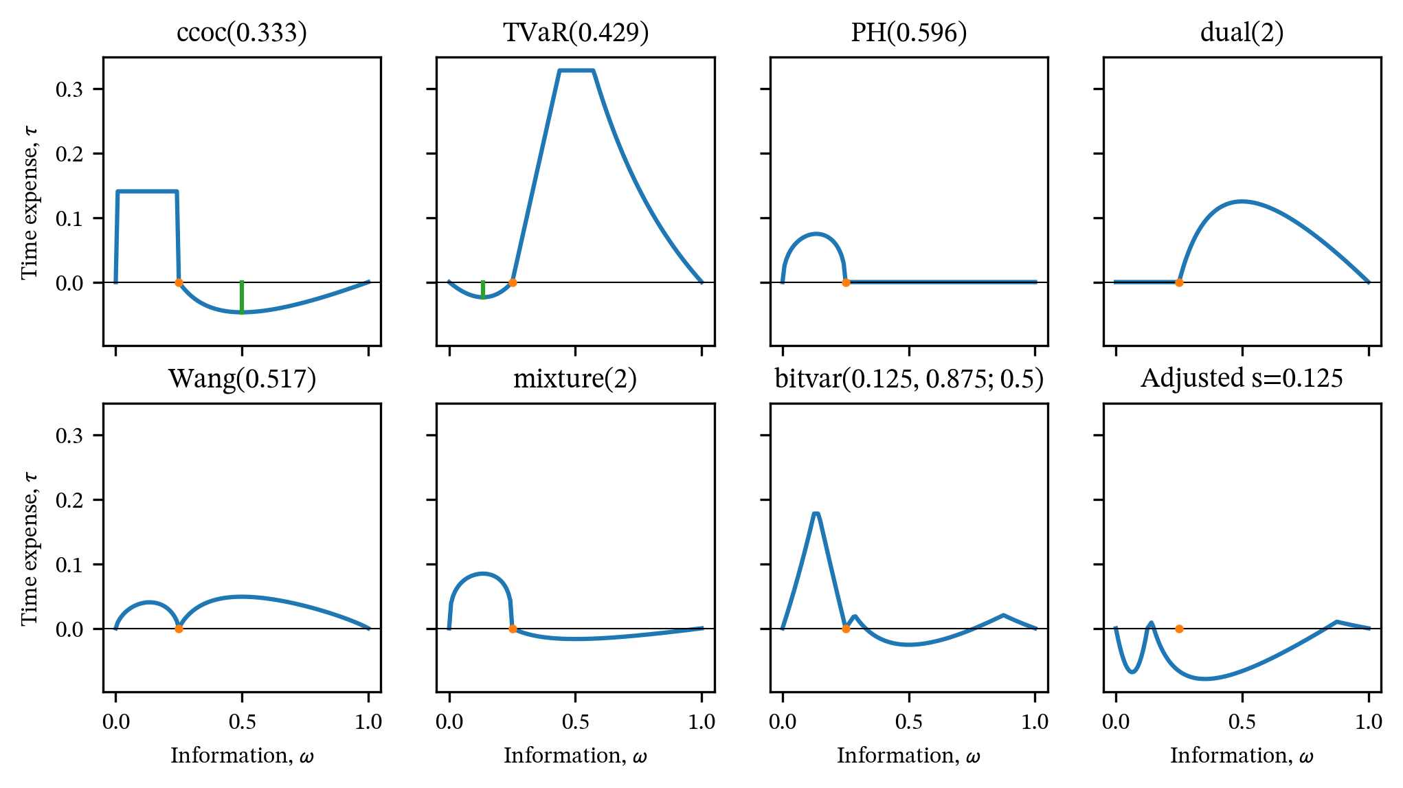
• Case 1: \(\omega_I < s\)
  • Information yields either a certain loss or a lower probability loss.
  • May be time cheap when the dual of the distortion is not super-multiplicative because \(\hat\rho(X)= 1-\check g\left(\displaystyle\frac{1-s}{1-\omega_I} \right)\check g(1-\omega_I)<1-\check g(1-s) = g(s)\).
  • Distortions that are not super-multiplicative are very expensive for higher probability events and have a high marginal cost with increasing risk. Thus there can be a time savings from information that combines a (relatively cheap) certain loss and combines it with a lower probability uncertain loss.
• Case 2: \(\omega_I > s\)
  • Information yields either a certain no-loss or a higher probability loss.
  • May be time cheap when the distortion is not sub if we can find \(\omega_I\) so that \(\hat\rho(X)=g(s/\omega_I)g(\omega_I)<g(s)\). This is not possible with sub-multiplicative.
  • Distortions that are not sub-multiplicative are very expensive for low probability events and have a low marginal cost with increasing risk. They bow up quickly and are then relatively flat. Thus there can be a time savings from information that allows to rule out the possibility of a loss and combines it with a higher probability uncertain loss.

“Perfect” information \(\omega=s\) reduces \(\hat\rho(X)=\rho(X)\) for Bernoulli risks, but for distortions that are either not sub-multiplicative or not super-multiplicative it may be possible to do better. However, uniformly across all Bernoulli risks, we can always find cases with time savings in these cases. This yields the following general formulation.

5.10.10 General results

Is this definition clear? See application in proof.

Definition 5.8 A distortion is simple Bernoulli time-expensive (simple BTE) if it is time expensive for all Bernoulli risks and all “simple” information defined by \((0,\omega]\) and \((\omega, 1]\).

Proposition 5.3 \(g\) is simple BTE if and only if \(g\) is sub-multiplicative and \(\check g\) is super-multiplicative.

Proof. \(g\) is simple BTE iff \(\hat\rho_{\omega_I}(X)\ge \rho(X)\) for all \(\omega_I\). Start with the (easier) case 2, where we require \[ g\left(\frac{s}{\omega_I} \right)g(\omega_I) \ge g(s) \] for all \(\omega_I \ge s\). But this holds precisely when \(g\) is sub-multiplicative, \(u=s/\omega_I\) and \(v=\omega_I\). (If it were not sub-multiplicative, we could construct a counter-example to simple BTE.)

In preparation for case 1, note that \(g(s)=1-\check g(1-s)\). Simple BTE in case 1 requires \[ \begin{aligned} & g\left(\frac{s-\omega_I}{1-\omega_I} \right)(1-g(\omega_I)) + g(\omega_I) \ge g(s) \\ \iff & \left(1-\check g\left(1-\frac{s-\omega_I}{1-\omega_I} \right)\right)(1-(1-\check g(1-\omega_I)) + 1 - \check g(1-\omega_I) \ge 1-\check g(1-s) \\ \iff & \left(1-\check g\left(1-\frac{s-\omega_I}{1-\omega_I} \right)\right)\check g(1-\omega_I) - \check g(1-\omega_I) \ge -\check g(1-s) \\ \iff & -\check g\left(\frac{1-s}{1-\omega_I} \right)\check g(1-\omega_I) \ge -\check g(1-s) \\ \iff & \check g(1-s) \ge \check g\left(\frac{1-s}{1-\omega_I} \right)\check g(1-\omega_I) \end{aligned} \] and the result follows.

5.10.11 Table of cases for BiTVaRs

*not oso

A general BiTVaR has two points of discontinuity \(s_1\) and \(s_0\), subject to:

• \(0 \leq s_1 \leq s_0 \leq 1\)
• \(k_1 > k_0\).

The corresponding distortion function \(g(s)\) is defined by \[ g(s) = \begin{cases} 0 & s = 0 \\ k_1 s & s \in (0, s_1] \\ s_1(k_1 - k_0) + k_0 s & s \in (s_1, s_0] \\ 1 & s \in (s_0, 1] \end{cases}. \]

Now, testing \(g(u)g(v)\) against \(g(uv)\), there are 10 possible cases for \(uv\), \(u\), and \(v\): they can be in each of the three intervals:

• \([0, s_1]\)
• \((s_1, s_0]\)
• \((s_0, 1]\)

Table tbl-bitvar-sub-multiplicative enumerates the possible cases.

Table 5.3: Ten cases for BiTVaR sub-multiplicativity.

Case	Interval for \(uv\)	Interval for \(u\)	Interval for \(v\)	\(g(uv)\)	\(g(u)g(v)\)	OK	Conclusion	Explanation
1	\([0, s_1]\)	\([0, s_1]\)	\([0, s_1]\)	\(k_1 uv\)	\(k_1^2 uv\)	y	positive	\(k_1>1 \implies k_1^2>k_1\)
2	\([0, s_1]\)	\([0, s_1]\)	\((s_1, s_0]\)	\(k_1 uv\)	\(k_1 u \cdot [s_1(k_1 - k_0) + k_0 v]\)	y	positive	\(g(uv)=g(u)v\le g(u)g(v)\)
3	\([0, s_1]\)	\([0, s_1]\)	\((s_0, 1]\)	\(k_1 uv\)	\(k_1 u\)	y	positive	\(v\le 1\)
4	\([0, s_1]\)	\((s_1, s_0]\)	\((s_1, s_0]\)	\(k_1 uv\)	\([s_1(k_1 - k_0) + k_0 u] \cdot [s_1(k_1 - k_0) + k_0 v]\)		positive	See Case 4
5	\([0, s_1]\)	\((s_1, s_0]\)	\((s_0, 1]\)	\(k_1 uv\)	\([s_1(k_1 - k_0) + k_0 u]\)	y	positive	\(g(uv)\le g(v)\)
6	\([0, s_1]\)	\((s_0, 1]\)	\((s_0, 1]\)	\(k_1 uv\)	\(1\)	y	positive	obvious
7	\((s_1, s_0]\)	\((s_1, s_0]\)	\((s_1, s_0]\)	\(s_1(k_1 - k_0) + k_0 uv\)	\([s_1(k_1 - k_0) + k_0 u] \cdot [s_1(k_1 - k_0) + k_0 v]\)		positive	See Case 7
8	\((s_1, s_0]\)	\((s_1, s_0]\)	\((s_0, 1]\)	\(s_1(k_1 - k_0) + k_0 uv\)	\([s_1(k_1 - k_0) + k_0 u]\)	y	positive	\(g(uv)
9	\((s_1, s_0]\)	\((s_0, 1]\)	\((s_0, 1]\)	\(s_1(k_1 - k_0) + k_0 uv\)	\(1\)	y	positive	obvious
10	\((s_0, 1]\)	\((s_0, 1]\)	\((s_0, 1]\)	\(1\)	\(1\)	y	zero	obvious

Here are the details for cases 4 and 7. Note that case 7 is mutually exclusive with 6 and 9: you can have one or the other two, but not all three. Note that, by definition:

• \(k_0 = \displaystyle\frac{1 - w}{s_0}\)
• \(k_1 = k_0 + \displaystyle\frac{w}{s_1} = \displaystyle\frac{1 - w}{s_0} + \displaystyle\frac{w}{s_1}\)

Case 4 \(uv \in [0, s_1], u, v \in (s_1, s_0]\). Here, \(g(uv) = k_1 uv = \left( \displaystyle\frac{1 - w}{s_0} + \frac{w}{s_1} \right) uv\) and \(g(u) = s_1(k_1 - k_0) + k_0 u = w + \displaystyle\frac{1 - w}{s_0} u\), and similarly for \(g(v)\). Hence \[ \begin{aligned} g(u)g(v) &= \left( w + \frac{1 - w}{s_0} u \right) \cdot \left( w + \frac{1 - w}{s_0} v \right) \\ &= w^2 + w \frac{1 - w}{s_0} (u+v) + \frac{(1 - w)^2}{s_0^2} uv \end{aligned} \] Thus, \[ g(u)g(v) - g(uv) = w^2 + w \frac{1 - w}{s_0} (u+v) + uv \left( \frac{(1 - w)^2}{s_0^2} - \frac{1 - w}{s_0} - \frac{w}{s_1} \right) \] We can potentially run into trouble if the coefficient of \(uv\) on the right is negative: \[ \begin{aligned} & \qquad\qquad\quad \frac{(1 - w)^2}{s_0^2} < \frac{1 - w}{s_0} + \frac{w}{s_1} \\ \iff & \frac{1 - w}{s_0}\left(\frac{1 - w}{s_0} - 1\right) < \frac{w}{s_1} \\ \iff & \frac{(1 - w)(1-w-s_0)}{s_0^2} < \frac{w}{s_1} \\ \iff & s_1 < \frac{w}{1 - w} \frac{s_0^2}{1-w-s_0} \\ \end{aligned} \] which is easy to test.

Case 7: \(uv, u, v \in (s_1, s_0]\) Note \(uv\in (s_1, s_0]\) implies \(s_0^2 > s_1\), otherwise this case cannot occur. Here \(g(u) = s_1(k_1 - k_0) + k_0 u = w + \displaystyle\frac{1 - w}{s_0} u\). Therefore, \[ \begin{aligned} g(u)g(v) - g(uv) &= w^2 + w \frac{1 - w}{s_0} (u+v) + \frac{(1 - w)^2}{s_0^2} uv - \left( w + \frac{1 - w}{s_0} uv \right) \\ %&= w^2 + w \frac{1 - w}{s_0} (u+v) + \frac{(1 - w)^2}{s_0^2} uv - w - \frac{1 - w}{s_0} uv \\ &= -w(1-w) + w \frac{1 - w}{s_0} (u+v) + \frac{1 - w}{s_0} uv\left(\frac{1 - w-s_0}{s_0} \right) \\ &= -w(1-w) + \frac{1 - w}{s_0} \left(w(u+v) + uv\frac{1 - w-s_0}{s_0} \right) \\ &= w(1-w)\left[ -1 + \frac{u+v}{s_0} + \frac{uv}{s_0w} \left( \frac{1 - w-s_0}{s_0} \right) \right] \\ &= \frac{w(1-w)}{s_0^2}\left[ -s_0^2 + s_0(u+v) + \frac{uv}{w} (1 - w-s_0) \right]\\ &= \frac{1-w}{s_0^2}\left[ -s_0^2w + s_0(u+v)w + uv(1 - w-s_0) \right] \\ \end{aligned} \] Thus, sub-multiplicative requires \[ (1 - w - s_0 )uv - s_0w(u+v) -ws_0^2 \ge 0 \] which we want to hold for all \(u,v\) in the interval. To test, set \(f(u,v)=(1 - w - s_0 )uv - s_0w(u+v) -ws_0^2\). At an internal extreme point \[ \frac{\partial f}{\partial u} = (1 - w - s_0 )v - s_0w =0 \quad\text{and}\quad \frac{\partial f}{\partial v} = (1 - w - s_0 )u - s_0w =0 \\ \phantom{x}\\ \implies u=v = \frac{s_0w}{1 - w - s_0 } \in (s_1, s_0]. \] To be in the interval requires \[ s_0w/(1 - w - s_0) \le s_0 \\ \implies w/(1 - w - s_0) \le 1 \\ \implies w \le (1 - w - s_0) \\ \implies s_0 \le 1-2w \] and \[ s_0w/(1 - w - s_0) > s_1 \\ \implies s_0w<s_1(1 - w - s_0) = s_1 - ws_1 -s_0s_1 \\ \implies s_0(w + s_1) < s_1(1 - w) \\ \implies s_0< \frac{s_1(1 - w)}{s_1 + w} \\ \] The Hessian is \[ \begin{pmatrix} 0 & 1-w-s_0 \\ 1-w-s_0 & 0 \end{pmatrix} \] so the determinant is \(<0\) and the critical point is a saddle point.

Boundary conditions

• \(u=v=s_0\)
• \(u=v=s_1\)
• \(u=s_0, v=s_1\)
• \(u=s_1, v=s_0\)
• Hummmm.

Table tbl-bitvar-restrictions lists the parameter restrictions required for each case to occur.

Table 5.4: Restrictions on conditions for cases apply.

Case	Interval for \(uv\)	Interval for \(u\)	Interval for \(v\)	Condition on \(s_1\) and \(s_0\)	Conflicts
1	\([0, s_1]\)	\([0, s_1]\)	\([0, s_1]\)	No condition needed
2	\([0, s_1]\)	\([0, s_1]\)	\((s_1, s_0]\)	No condition needed
3	\([0, s_1]\)	\([0, s_1]\)	\((s_0, 1]\)	No condition needed
4	\([0, s_1]\)	\((s_1, s_0]\)	\((s_1, s_0]\)	No condition needed
5	\([0, s_1]\)	\((s_1, s_0]\)	\((s_0, 1]\)	No condition needed
6	\([0, s_1]\)	\((s_0, 1]\)	\((s_0, 1]\)	\(s_1 > s_0^2\)	Exclusive with 7
7	\((s_1, s_0]\)	\((s_1, s_0]\)	\((s_1, s_0]\)	\(s_0^2 > s_1\)	Exclusive with 6 and 9
8	\((s_1, s_0]\)	\((s_1, s_0]\)	\((s_0, 1]\)	No condition needed, since \(s_0 > s_1 > s_1^2\)
9	\((s_1, s_0]\)	\((s_0, 1]\)	\((s_0, 1]\)	\(s_1 > s_0^2\)	Exclusive with 7
10	\((s_0, 1]\)	\((s_0, 1]\)	\((s_0, 1]\)	No condition needed

5.10.12 Properties of P2P Price

We can now describe the P2P price. We assume that \(T=2\) and at \(t=1\) information represented by a random variable \(I\) is revealed and \(\mathscr F_1=\sigma(I)\). The distribution of \(I\) under \(\mathsf P\) is \(\mu\). We use the following terminology. AV stands for actuarial (objective) expectation and MV for market value computed using \(\rho\). The difference is the risk adjustment.

1. \(\mathsf E[X]=\mathsf E[\mathsf E[X\mid I]]\) equals the \(t=0\) actuarial value of the liability at \(t=0\), sometimes called the objective expected loss or loss pick.
2. \(\rho(\mathsf E[X\mid I], \mu)\) equals the \(t=0\) market value of the \(t=1\) actuarial liability (MV.AV).
3. \(\mathsf E[\rho(X, P_I)]\) equals the \(t=0\) actuarial value of the \(t=1\) market value liability (AV.MV). This quantity equals the loss pick in the P2P. This is the \(t=0\) expected cost of transferring the risk in the second period, based on the information available at the end of the first period.
4. \(\rho(\rho(X, P_I), \mu)\) equals the \(t=0\) P2P, the premium to buy a premium value given by the \(t=0\) market value of the \(t=1\) market value liability (MV.MV). It is the \(t=0\) cost to secure a policy that will cover the cost of purchasing a second policy at \(t = 1\) on the risk emerging in the second period, taking into account the risk adjustments based on the information \(I\).
5. \(\rho(X)=\rho(X,\mathsf P)\) equals the \(t=0\) market value of \(X\) if it were a one-period risk. This value represents the price determined by applying the spectral risk measure to the distribution of \(X\), considering it as a risk over a single period without any interim evaluation or additional information.

Use the notation \(\rho^\star(X)\) for the P2P premium in (d).

These interpretations rely on the decomposition of \(\mathsf P\) into a mixture of conditional probabilities: \(\mathsf P\) is a mixture of \(\mathsf P_I\) over \(\mu\).

Often the information \(I\) is numeric and part of the ultimate \(X\). Case reserves are an example. We call this the A+B interpretation: \(X=A+B\) where \(A\) is the information. Notice that \(A\) is generally not \(\mathsf E[X\mid A]\), however, the general case be brought into this form by taking \(A=\mathsf E[X\mid I]\) and \(B=X-A\).

Theorem 5.2 (P2P Value.) The values defined above satisfy the following inequalities:

1. \(\mathsf E[X] \le \rho(\mathsf E[X\mid I], \mu) \le \rho(X)\):  MV of AV is at most one-period MV

2. \(\mathsf E[X] \le \mathsf E[\rho(X, P_I)] \le \rho(X)\):   AV of MV is at most one-period MV

3. In the A+B interpretation, if \(I=A\) and \(B\) independent then

   1. \(\rho^\star(X) = \rho(A) + \rho(B)\).
   2. \(\rho(X) \le \rho^\star(X)\): the P2P is at least the one-period MV.

4. If \(\max(A+B)=\max(A) + \max(B)\) and \(g\) is the constant cost of capital distortion then the P2P and one-period values are equal: \(\rho(X) = \rho(\rho(X, P_I), \mu)\).

Proof. The left-hand inequalities in (1-4) follow because a SRM always includes a non-negative risk margin, REF.

(1) follows from (Föllmer and Schied 2016, Cor 4.65), which says \(\rho(\mathsf E[X\mid \mathscr F])\le \rho(X)\). This is a consequence of \(\mathsf E[X\mid \mathscr F]\) being second-order stochastically dominated by \(X\) (almost the definition, STOYAN, ref, and Strassen (1965)) and that SRMs preserve SSD (nice REF). (Continuity? Or just ruling out the really weird behavior?)

(2) follows from Fubini’s theorem and Jensen’s inequality, see Bielecki et al. (2024) REF and spell out here.

(3.a) Going back to the definition, if \(A\) and \(B\) are independent then \(X_1 = \mathsf E[A+B\mid A] = A + \mathsf E[B]\). The decomposition by time period is \[ X = X_1 + (X - X_1) = A + \mathsf E[B] + (A + B - A - \mathsf E[B]) = A + (B - \mathsf E[B]) \] Therefore, the second-period policy MV equals \(A + \mathsf E[B] \rho(B - \mathsf E[B]) = A + \rho(B)\). Applying \(\rho\) gives the P2P premium of \(\rho(A) + \rho(B)\) by cash invariance. (8.b) follows because \(\rho\) is subadditive.

(4) Let \(g(s) = sv + d\) be a CCoC distortion, where \(r = d / v\) is the constant cost of capital, \(d+v=1\). Then CCoC pricing \(\rho(X) = s\mathsf E[X] + d\max(X)\) is additive under the assumption for maximum values. Thus (4) follows from (3.a).

Item (3.a) confirms the intuition that slowly emerging risks should cost more, but only in the independent case. Example REF shows that multi-period risk emergence can lower the cost when \(A\) and \(B\) are not independent.

Item (4) applies when \(A\) and \(B\) are independent. It produces two different risk-adjusted distributions with the same mean, see the examples below.

The relations between \(\rho(\mathsf E[X\mid I])\) and \(\mathsf E[\rho(X(P_i))]\), and \(\rho(X)\) and \(\rho^\star(X)\) are indeterminate, as shown in examples below. These also show that the convolution of \(\mu^g\) and the \(g\)-risk adjusted distribution of \(B\) suggested by (3.b) does not equal the distribution \(P^g\), despite the two distributions having the same means.

Relationship to Solvency II coc rm…. vs (4)?

---

This section introduces some new or less common terminology. sec-examples then gives some examples to illustrate the behaviors that ensue to motivate our more general results. These are stated and proved in sec-results.

Definition 5.9 A distortion function \(g\) is sub-multiplicative if \(g(st)\le g(s)g(t)\) for all \(s,t \in[0,1]\).

Definition 5.10 Given a spectral risk measure \(\rho\) associated to the distortion function \(g\) and a sub-sigma algebra \(\mathscr F_1\subseteq \mathscr F\) define the conditional risk measure given \(\mathscr F_1\) to be \[ \rho(X\mid \mathscr F_1)(\cdot) = \int_{[0,\infty)} g(\Pr(X>x\mid \mathscr F_1)(\cdot)) - \int_{(-\infty, 0)} (g(\Pr(X>x\mid \mathscr F_1)(\cdot))-1)\,dx. \]

Add to results: Bielecki result that this comes from an expectation…

Definition 5.11 The P2P functional associated with a single-period risk measure \(\rho\) and a sub-sigma algebra \(\mathscr F_1\subseteq \mathscr F\) is given by \[ \hat\rho(X) = \rho(\rho(X\mid \mathscr F_1)) \] where \(\rho(X\mid \mathscr F_1)\) is the conditional risk measure given \(\mathscr F_1\).

If there is ambiguity about \(\mathscr F_1\) in the definition of \(\hat\rho\), then write \(\hat\rho_{\mathscr F_1}\). If \(\mathscr F_1=\sigma(N)\) is generated by a random variable or vector \(N\), then write \(\hat\rho_N\).

Definition 5.12 Given a single-period risk measure \(\rho\) and a risk \(X\), we say \(X\) is time expensive (for \(\rho\) and \(\mathscr F_1\)) if \(\hat\rho(X)\ge \rho(X)\) and time cheap if \(\hat\rho(X)<\rho(X)\). The time expense \(\mathcal T(X)=\hat\rho(X) - \rho(X)\). If the time expense is negative we call it the time savings.

5.11 The \(m\)-Stable Assumption

posts/050-files/m-stable.qmd

5.11.1 Technical Results

This section provides a summary of key technical results for dynamic (intertemporal) risk measures.

We work on a filtered probability space (\(\Omega,\mathcal F,(\mathcal F_t)_{t=0,\dots,T},P\)). A terminal (discounted) loss is an \(\mathcal F_T\)-measurable random variable \(X\).

A dynamic coherent risk measure is a family \({\rho_t}_{t=0}^T\) with \(\rho_t: L^\infty(\mathcal F_T) \to L^\infty(\mathcal F_t)\) satisfying, for each \(t\):

1. monotonicity: if \(X \le Y\) then \(\rho_t(X) \ge \rho_t(Y)\),
2. cash additivity: for any \(\mathcal F_t\)-measurable \(m\), \(\rho_t(X+m)=\rho_t(X)-m\),
3. positive homogeneity and subadditivity (or convexity in the convex case). These are the natural intertemporal analogues of coherent (resp. convex) risk measures in the static one-period sense of Artzner et al. [Artzner, Delbaen, Eber, Heath 1999]. Coherent is often assumed for clarity; convex versions behave similarly but with penalties instead of sets of measures. See e.g. Föllmer & Schied 2002/2004.

The dual representation is central. For coherent \(\rho_t\), one can write \[ \rho_t(X) = \operatorname{ess,sup}_{Q \in \mathcal D_t} Q(-X \mid \mathcal F_t), \] where \(\mathcal D_t\) is a (possibly random) set of probability measures \(Q\) on (\(\Omega,\mathcal F_T\)) absolutely continuous w.r.t. \(P\), and \(Q(-X \mid \mathcal F_t)\) is the conditional expectation of \(-X\) under \(Q\). The sets \(\mathcal D_t\) are often called the scenario sets (test measures, stress measures, or priors). See Delbaen 2006; Delbaen, Peng & Rosazza Gianin 2010; Kupper & Schachermayer 2009.

This dual form is analogous to the static one-period representation \[ \rho(X) = \sup_{Q \in \mathcal D} Q(-X), \] but now conditional.

5.11.2 Time consistency and the tower property

A crucial axiom for intertemporal use is time consistency (a.k.a. dynamic consistency). The strongest and most commonly studied version in this literature is:

For all \(s<t\), \[ \rho_s(X) = \rho_s\big(-\rho_t(X)\big). \]

Equivalently, for all \(s<t\), if \(\rho_t(X) \le \rho_t(Y)\) (a.s.) then \(\rho_s(X) \le \rho_s(Y)\). This rules out preference reversals when you roll the risk assessment back in time. This is the nonlinear analogue of the tower property for conditional expectation. See Artzner, Delbaen, Koch-Medina 2009; Kupper & Schachermayer 2009.

Time consistency is not automatic. If you simply “bootstrap” a one-period coherent risk measure forward in time and define \(\rho_t\) recursively by evaluating one-step-ahead P&L with the same static rule at each date, you generally do not get time consistency. You instead get dynamic preference reversals and horizon anomalies.

The literature shows that time consistency and the structure of \({\mathcal D_t}\) are in fact equivalent, through what is called m-stability.

5.11.3 m-stability (stability under pasting)

Fix \(t\). Take any two measures \(Q^1,Q^2 \in \mathcal D_t\). Consider a stopping time \(\tau \ge t\), and consider the “pasted” measure \(Q^*\) that behaves like \(Q^1\) up to \(\tau\), and then, conditional on \(\mathcal F_\tau\), switches and behaves like \(Q^2\) on the continuation. More generally, allow \(\tau\) to have multiple branches and allow different choices of continuation measure branch by branch. This operation is sometimes described as pasting or concatenation. Intuitively: we are allowed to choose, at each future node, whichever continuation scenario is worst in that node, and stitch those nodewise-worst conditionals into a single global measure.

The set \(\mathcal D_t\) is called m-stable if it is closed under all such pastings: whenever you paste admissible \(Q\)’s along stopping times, you stay in \(\mathcal D_t\). See Delbaen 2006; Delbaen, Kupper & Schachermayer 2004/2006; Kupper & Schachermayer 2009.

The main structural theorem is:

• For coherent dynamic risk measures, strong time consistency (the tower property above) is equivalent to m-stability (or stability under pasting) of the representing sets \(\mathcal D_t\). In other words, \(\rho_s(X) = \rho_s(-\rho_t(X))\) for all \(s<t\) if and only if, for each \(t\), \(\mathcal D_t\) is stable under attaching, node by node, worst-case future conditionals and these pasted measures remain admissible. See Delbaen 2006; Kupper & Schachermayer 2009.

Economic reading: time consistency means you can precommit at time \(s\) to the same “worst-case model of the world” that you will choose after you learn more information at later times \(t>s\). m-stability is exactly the formalization of “I can precommit to that.” If \(\mathcal D_t\) is not m-stable, you get dynamic preference reversals and loss of any coherent tower property.

In the language of Epstein & Schneider (2003), this same structural requirement is called rectangularity. Rectangularity says: the set of ambiguous priors is a product set across dates/histories, so that for each history you can pick the worst continuation independently, and the stitched global prior is still admissible. Epstein & Schneider prove: recursive multiple-prior (Gilboa–Schmeidler style) preferences are dynamically consistent if and only if the set of priors is rectangular. This is the same idea as m-stability, translated from finance risk-measure language into ambiguity-averse utility language. See Epstein & Schneider 2003; also Epstein & Schneider 2007.

So: m-stability (Delbaen/Kupper/Schachermayer) iff rectangularity (Epstein/Schneider) iff strong time consistency.

5.11.4 Law invariance, distortion risk measures, and failure of m-stability

Many coherent capital measures used in practice are law invariant (they depend only on the distribution of \(X\) under \(P\)) and comonotonic additive (if \(X\) and \(Y\) are comonotone, \(\rho(X+Y)=\rho(X)+\rho(Y)\)). By a classic result, static coherent, law-invariant, comonotone-additive risk measures are exactly the distortion (a.k.a. spectral) risk measures \[ \rho(X) = \int_0^1 \text{VaR}_u(X), dg(u) \] for some increasing concave distortion \(g\). Tail Value-at-Risk / Expected Shortfall is a canonical special case, with \(g(u) = \min(u/\alpha,1)\) for tail level \(\alpha\). See Acerbi 2002; Wang, Young & Panjer 1997; Wirch & Hardy 1999.

These spectral/distortion functionals admit dual sets \(\mathcal D\) that can be described as all \(Q\) whose Radon–Nikodym densities w.r.t. \(P\) lie in a certain “tilted tail” envelope; for ES at level \(\alpha\), one gets \(dQ/dP \le 1/\alpha\) and \(PQ=1\). See Delbaen 2002; Acerbi 2002.

Now ask: if we try to turn such a static \(\rho\) into a dynamic \(\rho_t\) via \[ \rho_t(X)=\operatorname{ess,sup}_{Q\in\mathcal D} Q(-X\mid \mathcal F_t), \] using the same \(\mathcal D\) at all times, is \({\rho_t}\) time consistent?

Answer from the literature: no, except in degenerate cases. The associated \(\mathcal D\) for any genuinely nonlinear distortion is not m-stable. Intuitively, these \(\mathcal D\) allow you to overweight tail states “a lot but not infinitely.” When you move one step forward in time and condition on new information, the dynamically worst continuation typically behaves as if “conditional on this branch, the catastrophic tail happens with probability 1.” That conditional is more extreme than anything globally allowed in \(\mathcal D\), which only allows bounded tilts, not full concentration. Because \(\mathcal D\) is not closed under pasting these extreme local conditionals into a single global measure, m-stability fails, and thus time consistency fails. See Kupper & Schachermayer 2009; Acciaio & Penner 2011.

This is exactly why familiar tail-focused capital formulas like Expected Shortfall (ES) / TVaR are dynamically inconsistent: they violate m-stability. Iterating ES across time does not satisfy the tower property and leads to preference reversals. The same is true for essentially all nontrivial spectral (distortion) risk measures.

There are only two “distortions” \(g\) that do give m-stability:

1. \(g(u)=u\). Then \(\rho(X)=P(-X)\) (i.e. minus the P-expectation of \(X\)). The dual set is \(\mathcal D={P}\). This is trivially m-stable and yields \(\rho_t(X)=P(-X \mid \mathcal F_t)\), which is linearly time consistent by the usual tower property of conditional expectation. Economically this is risk-neutral valuation under a single fixed measure. See Föllmer & Schied 2002; Kupper & Schachermayer 2009.

2. The “worst case” (essential supremum) distortion \(g(u)=1_{{u>0}}\) in the limit. Then \(\rho(X)=\operatorname{ess,sup}(-X)\). The dual set \(\mathcal D\) contains all Dirac-like extreme measures, which is closed under pasting by construction, hence m-stable. The dynamic version is conditional essential supremum, which is again time consistent. Economically this is maximal ambiguity aversion / robust control. See Föllmer & Schied 2002; Kupper & Schachermayer 2009; also references in Epstein & Schneider 2003 on max–min preferences.

Everything in between — i.e. any distortion that is genuinely tail-averse but not “infinite worst-case” and not linear expectation — fails m-stability and therefore fails strong time consistency.

This is consistent with broader law-invariance impossibility theorems: if you demand law invariance, cash additivity, coherence, and strong time consistency on a sufficiently rich (non-atomic) probability space, then either the dynamic risk measure collapses to conditional expectation under some fixed measure, or it collapses to a worst-case (essential supremum–type) operator. There is no genuinely spectral, tail-weighted, comonotonic-additive, law-invariant dynamic coherent risk measure that is also strongly time consistent. See Kupper & Schachermayer 2009; Kupper & Schachermayer 2011; Delbaen 2021.

5.11.5 Comonotonicity and Delbaen 2021

Delbaen (2021) isolates and sharpens this tension: suppose \({\rho_t}\) is a dynamic coherent risk measure that is

1. time consistent in the strong sense above,
2. comonotonic additive at each time \(t\).

Then \(\rho_t\) must in fact be (conditionally) linear expectation under some measure \(Q_t\); in particular, you essentially fall back to a linear pricing functional. In other words, you cannot simultaneously have (i) strong time consistency, (ii) coherent risk aversion that is (iii) comonotonic additive in the usual actuarial sense, unless you give up true nonlinearity. See Delbaen 2021.

This recovers the intuition: time consistency is brutally strong. If you also want comonotonic additivity — a property beloved in static actuarial capital allocation — you are forced into linear/conditional-expectation-type functionals. Nonlinear tail loadings and dynamically consistent comonotonic additivity cannot coexist except in degenerate/worst-case limits.

5.11.6 Interpretation in preference theory (Epstein–Schneider)

In Epstein–Schneider (2003) on recursive multiple-priors utility, a decision maker evaluates continuation utility by taking the worst expected utility over a set \(\Pi\) of priors. Dynamic consistency (no preference reversals over time, analogous to the tower property) holds if and only if \(\Pi\) is rectangular. Rectangularity means: for each history, you can choose any continuation prior from a prescribed set of conditionals, independently across histories, and the stitched global prior is still in \(\Pi\). This is exactly the same structural requirement as m-stability in the finance / coherent risk measure setting. Epistemically: time consistency forces “statewise worst-case continuation with commitment.” Without rectangularity, you get dynamic inconsistency. See Epstein & Schneider 2003; Epstein & Schneider 2007.

So: rectangularity in Epstein–Schneider = m-stability of \(\mathcal D_t\) in Delbaen/Kupper/Schachermayer = strong time consistency for \({\rho_t}\).

5.11.7 Bottom line

1. Dynamic coherent risk measures can always be represented as conditional worst-case expectations over a family \(\mathcal D_t\) of scenario measures.

2. Strong time consistency (tower property, no preference reversals) iff m-stability of those scenario sets. m-stability = closure under pasting worst-case continuations node by node. This is exactly rectangularity in the Epstein–Schneider multiple-priors sense.

3. Standard actuarial/financial tail measures such as spectral (distortion) risk measures, including Expected Shortfall / TVaR, are not m-stable. Their \(\mathcal D\) is not closed under pasting. Therefore, if you iterate them through time in the obvious “apply the same rule each period” way, you do not get a time-consistent dynamic risk measure. You get capital processes and rankings that can flip across time.

4. The only distortions whose \(\mathcal D\) is m-stable are essentially:

   • the trivial linear distortion \(g(u)=u\), giving conditional expectation under a fixed measure (risk-neutral style), and
   • the degenerate worst-case distortion (conditional essential supremum). Everything “in between” fails m-stability.

5. Delbaen (2021) shows a deeper incompatibility: if you insist on both strong time consistency and comonotonic additivity in the dynamic setting, the only possibility is essentially conditional expectation (linear). In other words, once you demand full dynamic coherence (time consistency) plus static-style comonotonic capital additivity, you have ruled out genuinely nonlinear tail-risk loading.

6. Epstein–Schneider’s rectangularity result is the preference-theoretic mirror: dynamically consistent ambiguity aversion requires rectangular (pasting-stable) sets of priors. Non-rectangular ambiguity sets cause dynamic preference reversals for exactly the same structural reason.

The upshot for intertemporal risk measurement in insurance / finance is that there is a three-way trade-off:

• rich nonlinear tail aversion (spectral / distortion style, comonotonic allocation),
• strong time consistency / tower property,
• and non-degenerate (i.e. not purely worst-case, not purely linear) pricing.

You can really have at most two of these in a meaningful way, and in most practical tail-risk measures you only keep the first one. The technical backbone of that statement is precisely m-stability (Delbaen/Kupper/Schachermayer) and rectangularity (Epstein/Schneider).

5.11.8 Examples

See m-stable.ipynb for a starter set of examples. Just TVaR!

---

5.11.9 References

Acerbi, C. (2002). Spectral measures of risk. J. Banking & Finance 26, 1505–1518. Acerbi (2002)

Artzner, P., Delbaen, F., Eber, J.-M., Heath, D. (1999). Coherent measures of risk. Math. Finance 9, 203–228. Artzner et al. (1999)

Artzner, P., Delbaen, F., Koch-Medina, P. (2009). Risk measures and efficient use of capital. Astin Bulletin 39, 101–116. Artzner et al. (2009)

Delbaen, F. (2002). Coherent risk measures on general probability spaces. In: Advances in Finance and Stochastics, 1–37. Delbaen (2002)

Delbaen, F. (2006). The structure of m-stable sets and in particular of the set of risk neutral measures. In: In Memoriam Paul-André Meyer: Séminaire de Probabilités XXXIX, 215–258, Springer. Delbaen (2006) probably.

Delbaen, F., Kupper, M., Schachermayer, W. (2004, 2006). Coherent risk measures and m-stable sets of probability measures. (Working papers 2004; published variants in Stochastic Processes and their Applications 2008 and related volumes.)

Delbaen, F., Peng, S., Rosazza Gianin, E. (2010). Representation of the penalty term of dynamic concave utilities. Finance and Stochastics 14, 449–472. Delbaen et al. (2010)

Delbaen, F. (2021). Comonotonicity and time consistency. Finance and Stochastics 25, 215–241. Delbaen (2021)

Epstein, L. G., Schneider, M. (2003). Recursive multiple-priors. J. Economic Theory 113, 1–31. Epstein and Schneider (2003)

Epstein, L. G., Schneider, M. (2007). Learning under ambiguity. Rev. Economic Studies 74, 1275–1303. Epstein and Schneider (2007)

Föllmer, H., Schied, A. (2002, 2004). Convex measures of risk and trading constraints. Finance and Stochastics 6, 429–447. Also: Stochastic Finance, de Gruyter. Föllmer and Schied (2002)

Kupper, M., Schachermayer, W. (2009). Representation results for law invariant time consistent functions. Math. Finance 19, 599–619. (See also related 2011 follow-ups on law invariance and time consistency.)

Wang, S., Young, V. R., Panjer, H. H. (1997). Axiomatic characterization of insurance prices. Insurance: Mathematics and Economics 21, 173–183. Wang et al. (1997)

Wirch, J. L., Hardy, M. R. (1999). A synthesis of risk measures for capital adequacy. Insurance: Mathematics and Economics 25, 337–347. Wirch and Hardy (1999)

---

5.12 Information

posts/050-files/information.qmd

5.12.1 Data and Information

Raw data is both an oxymoron and a bad idea; to the contrary, data should be cooked with care. [Geoff Bowker NEED REF]

Quoted in, and a theme of, Gitelman (2013).

Actuaries typically treat data as a static snapshot: a triangle, a bordereau, a point-in-time extract. But data are just symbols. The information they contain is the sigma algebra they generate, the partition of possible worlds they allow us to distinguish. Two data items that look different can induce the same partition and thus carry the same information. A coded injury level and a free-text note may differ as data, yet if they separate claims into the same outcome buckets, they are informationally equivalent.

This clarifies Bowker’s observation that “raw data is an oxymoron.” Any observation presupposes a way of carving up the world: categories, measurement systems, and institutional conventions. In sigma-algebra terms, there is no raw data because the act of recording data already selects a partition of the sample space. Information is that partition; data are one representational slice through it.

A further distinction matters. Information describes the entire structure of possibilities—every atom of the partition that could conceivably be observed in this modelling framework. Data is a single realized point within that structure. When we observe \(Y=y\), we do not learn the world; we only learn that the world lies in one atom of \(\sigma(Y)\). Information is therefore broader and more abstract: it defines the space of potential observations and the distinctions the model can draw.

This sits alongside a deeper tension. All of these definitions rely on an underlying sample space \(\Omega\), but in domains like insurance, medicine, and economics the true space of possibilities is too large and open-ended to specify. Gilboa (2015) emphasizes this point: decision makers in such settings face vast, ill-defined state spaces rather than the controlled ones of the physical sciences. The sample space exists only as a modelling device, and information is always relative to that model rather than to the world itself. The contrast between well defined events in catastrophe models versus nebulous casualty model samples spaces illustrates this tension.

For actuaries, the consequence is that data are not fixed objects but manifestations of an evolving informational process. As a claim develops, new observations refine the partition of \(\Omega\), shrinking the uncertainty around ultimate loss. What we are really modelling is the emergence of information through time; the data are simply its current encoding.

Remark 5.4 (TL;DR).

• Data are symbols, observations, raw values.

• Information is the sigma algebra generated by the data, i.e., the measurable partition of the state space you obtain after observing the data.

5.12.2 Information Descriptors

The importance and complexity of the concept of information is illustrated its many descriptors. We can speak of information’s intrinsic

• accessibility: ability to obtain it
• accuracy: closeness to truth
• ambiguity: degree of multiple interpretations
• authority: recognized legitimacy
• bias: systematic distortion
• clarity: ease of comprehension
• cognitive load: processing demand
• coherence: internal consistency
• completeness: coverage of relevant states
• compressibility: ability to reduce without loss
• decay: loss of relevance
• dimensionality: number of variables or features
• distinctiveness: contrast with background
• entropy: Shannon uncertainty
• format: symbolic, numeric, linguistic, spatial
• granularity: resolution, fineness
• hierarchy: levels, layers, nestedness
• meaning: semantic content
• memorability: retention likelihood
• novelty: departure from prior understanding
• provenance: source quality
• refresh rate: arrival frequency
• reliability: consistency across measurements
• specificity: how targeted the content is
• stability: robustness against new observations
• structure: degree of organization
• timeliness: latency, recency
• transparency: openness of method and data
• validity: measures what it claims to measure
• verifiability: ability to check correctness
• volatility: rate of change
• volume: amount, size

In addition, information has relational descriptors relative to a target variable or decision. For a given decision, information can have

• importance: how much conditioning on the information changes the distribution of the target
• precision: dispersion of estimates of the target
• relevance: how strongly the information explains variation in the target
• salience: predictive significance for the target
• signal-to-noise ratio: useful vs irrelevant fluctuation for prediction
• sufficiency: statistical sufficiency for a parameter or distribution
• tail sensitivity: how much the information improves inference about extreme outcomes
• value: expected decision value; expected value of perfect and sample information (EVPI/EVSI)

To actuaries, granularity and importance are especially central, because together they determine how an information state refines the sigma algebra relevant to the prediction of ultimate loss.

5.12.3 Decision Theory Terminology

Information enables decisions and management is decision making with incomplete information: exactly the subject of decision theory. In the theoretic model there is a sample space of random states of the world, usually denoted \(\omega \in \Omega\). Everything derives from the state:

• \(\omega\in\Omega\) is the true, unknown state of the world.
• \(X = X(\omega)\) is the outcome you care about (e.g., ultimate loss).
• \(Y = Y(\omega)\) is the data or signal you observe.
• \(\mathcal{G} = \sigma(Y)\) is the sigma algebra of information generated by the data/signal \(Y\).
• \(a\) is an action selected using the data \(Y\) from a set of possible actions \(A\).
• A decision rule is a \(Y\)-measurable mapping \[ a:\Omega \to A\qquad \omega\mapsto \phi(Y(\omega)) \] for some measurable function \(\phi\).
• \(L(a, X)\) is the loss function random variable giving loss from selecting action \(a\) for outcome \(X\); in state \(\omega\) the loss is \(L(a(\omega), X(\omega)) = L(a,X)(\omega)\).
• A decision problem: given a state space \(\Omega\), with a probability \(\mathsf P\), an outcome \(X:\Omega\to\mathbb R\), data or signal \(Y\) generating information \(\mathcal G=\sigma(Y)\), a set of actions \(A\), a loss function \(L:A\times \mathbb R\to\mathbb R^+\), and a decision rule which we take to be minimize expected loss, the problem is to determine the \(Y\)-measurable function \(a:\Omega\to A\) that minimizes the \(\mathsf PL(a,X)\).

The decision rule makes it clear that you choose the action after seeing the signal. You do not see \(X\). \(L\) uses the loss sign convention: loss is positive and larger is worse. You want to minimize loss.

To solve the decision problem given information \(\mathcal{G}\) and outcome \(X\), means finding the \(\mathcal{G}\)-measurable action rule \(a\) that minimizes expected loss \[ \mathsf{P}(L(a(\omega), X(\omega))). \] This is the best strategy allowed by the information \(\mathcal{G}\), because \(a(\omega)\) can only depend on \(\mathcal{G}\), not on the full \(\sigma(X)\). The expectations is unconditional and hence is a number.

Remark 5.5 (TL;DR).

• State = underlying \(\omega\).
• Outcome = random variable \(X(\omega)\).
• Data or signal = \(Y = Y(\omega)\) that you observe.
• Information = sigma algebra \(\mathcal{G}=\sigma(Y)\) generated \(Y\).
• Action = \(\mathcal{G}\)-measurable function \(a(\omega)\).
• A decision rule = minimize expected loss, for example.
• Solving the decision problem = choose the \(\mathcal{G}\)-measurable \(a\) that minimizes expected loss \(\mathsf P(a, X)\).
• Blackwell dominance = optimal loss under \(\mathcal{G}_1\) is \(\le\) roptimal loss under \(\mathcal{G}_2\) for all possible decision problems.
• Equivalence = this is true iff \(\mathcal{G}_2\) is a garbling of \(\mathcal{G}_1\) (coarser partition).

All the ingredients \((\Omega, \mathcal F, \mathsf P, X, Y, A, L)\) define a decision problem.

Statements about decision problems usually assume \((\Omega, \mathcal F, \mathsf P)\) are fixed and are then universal over the remaining unspecified parts. For example, the statement that “for every decision problem, \(\mathcal{G}_1\) never yields worse expected loss than \(\mathcal{G}_2\)” means:

• For every loss function \(L\),
• every distribution of \((X,Y_1,Y_2)\),
• and every action set \(A\),
• the optimal \(\mathcal{G}_1\)-measurable rule achieves expected loss \(\le\) the optimal \(\mathcal{G}_2\)-measurable rule.

Equivalently: The best you can do using \(\mathcal{G}_1\) is always at least as good as the best you can do using \(\mathcal{G}_2\). This gives a decision-theoretic definition of more informative.

Blackwell’s decision theory says that finer information implies a bigger set of admissible rules and hence weakly lower minimal expected losses. This is the deterministic case.

However, Blackwell moves beyond this, to consider decision making based on noisy data. The classical sigma-algebra view treats information as deterministic: you observe \(Y=f(\omega)\), and the sigma algebra \(\sigma(Y)\) determines what you know. Blackwell generalized this to allow for noisy signals: an experiment is any Markov kernel \(K(\omega,\cdot)\) giving the distribution of observations conditional on the true state. This is essential for real-world settings, including insurance, where observations about a claim are always imperfect and carry stochastic error. In this setting, “more informative” means: for every decision problem, the optimal expected loss using experiment \(K_1\) is no worse than using \(K_2\); equivalently, \(K_2\) can be obtained by garbling (adding noise to) \(K_1\).*

If the observation \(Y\) itself may be noisy, and all that matters is the conditional distribution of \(Y\) given the true state \(\omega\). Formally:

• An experiment is a Markov kernel \[ K(\omega, \cdot)=\mathsf{P}(Y\in\cdot\mid \omega). \]
• A decision rule is any function of the observed \(Y\), not \(\omega\).
• Two experiments can be compared even if both are noisy.

Now, experiments are typically not refinements of one another and the sigma-algebra \(\sigma(Y)\) does not capture the information in the experiment because the distribution of \(Y\mid\omega\) is what matters not the raw value of \(Y\).

Blackwell’s dominance criterion reflects this generality. Two experiments \(K_1\) and \(K_2\): \[ K_1 \text{ dominates } K_2 \iff K_2 = K_1 M \text{ for some Markov kernel } M \] (\(K_2\) is a garbling of \(K_1)\). So if the output of experiment 2 can be produced by taking the output of experiment 1 and adding extra noise, then experiment 1 is strictly more informative. This is exactly garbling. The deterministic case reduces to sigma-algebra refinement, but in the noisy case, refinement must be understood probabilistically, not structurally.

All our actuarial data are noisy signals of a latent truth.

5.12.4 Strassen vs Blackwell

A garbling is a Markov kernel \[ Y \to Z, \] meaning we observe \(Z\) which is a noisy, coarsened, or scrambled version of \(Y\). Key properties:

• \(X \to Y \to Z\) is a Markov chain
• \(\sigma(Z)\) is coarser than \(\sigma(Y)\)
• \(Z\) contains no more information about \(X\) than \(Y\) does

Garbling is information degrading. In economic language: push \(Y\) through a noisy channel.

Strassen (1965) is about martingale couplings and equivalently convex order: \[ X \preceq_{\text{cx}} Y \quad\Longleftrightarrow\quad \exists; (X,Y) \text{ such that } \mathrm{P}X(Y\mid X) = X. \]

Interpretation:

• \(Y\) is a “mean-preserving spread” of \(X\)
• \(Y\) is less informative than \(X\) in the sense of risk
• AND \(X\) can be recovered as \(\mathsf{P}(Y\mid X)\)

This is noise adding.

If \(Y = X + \epsilon\) with \(\mathsf{P}(\epsilon\mid X)=0\), then \(Y\) is a mean-preserving spread (one special case). But: convex order is much weaker than literal additive noise.

The connection

• Garbling: makes a signal coarser, less informative, destroys structure; it degrades information and destroys the ability to distinguish states

• Strassen: characterizes when one variable is a noisy version of another in convex order; it degrades the sharpness or concentration of a distribution.

• Garbling is sigma-algebra dilution; Strassen is distributional dilution.

Martingales preserve means but increase dispersion; garblings preserve decision value but reduce information.

In full generality, a statistical experiment is a Markov kernel that produces a noisy observation of the underlying state, and Blackwell’s dominance relation is defined in that general setting. For our purposes, we work with deterministic information states generated by sigma algebras. This is sufficient because the InformationSimulator deals with idealized information partitions—FNOL triage, injury buckets, legal involvement, medical updates—that can be represented cleanly as refinements of a deterministic signal. If one wished to incorporate misclassification or measurement error, the kernel-based version would be required, but we do not pursue that here.

Expected Value of Perfect Information (EVPI)

Definition EVPI is the improvement in expected performance if you knew \(X\) before choosing the decision.

Formally:

1. Without extra information, choose \[ a_0 = \arg\min_a\ \mathsf{P}( L(a,X) ). \]

2. With perfect information (i.e., conditioning on \(\sigma(X)\)), you choose a different action for each \(X\): \[ a^*(X) = \arg\min_a L(a,X). \]

3. EVPI is \[ \mathrm{EVPI} = \mathsf{P}\big( L(a_0,X) \big) ;-; \mathsf{P}\big( L(a^*(X),X)\big). \]

Interpretation: the maximum possible value of any information—how much you gain if uncertainty disappears entirely.

Expected Value of Sample Information (EVSI)

EVSI evaluates partial or imperfect information, like medical notes, FNOL data, legal involvement, etc.

Let \(I\) be the information (a random variable or sigma algebra).

1. With \(I\), choose \[ a_I = \arg\min_a\ \mathsf{P}( L(a,X) \mid I ). \]

2. EVSI is \[ \mathrm{EVSI} = \mathsf{P}\big( L(a_0,X) \big) ;-; \mathsf{P}\big( \mathsf{P}( L(a_I,X)\mid I ) \big). \]

Interpretation: the expected improvement in decisions from learning \(I\) before acting.

Relationship to sigma algebras

If \(I_1\) and \(I_2\) correspond to sigma algebras \(\mathcal{G}_1 \supseteq \mathcal{G}_2\), then Blackwell dominance implies:

• \(\mathrm{EVSI}(I_1)\ge \mathrm{EVSI}(I_2)\)
• and \(\mathrm{EVPI}\ge\mathrm{EVSI}(I_1)\)

because more information produces finer conditional expectations and lower conditional losses.

Insurance example (simplified)

Let \(X\) be ultimate claim severity and let \(a\) be the reserve. Use quadratic loss \(L(a,X)=(a-X)^2\).

Then:

• Without information, \(a_0 = \mathsf{P}(X)\)
• With partial info \(I\), \(a_I = \mathsf{P}(X\mid I)\)
• With perfect info, \(a^*(X)=X\)

Compute:

1. EVPI = \(\mathsf{P}\big[(\mathsf{P}(X)-X)^2\big]\) = unconditional variance of \(X\).

2. EVSI = unconditional variance minus expected conditional variance: \[ \mathrm{EVSI} = \mathrm{Var}(X) - \mathsf{P}( \mathrm{Var}(X\mid I) ). \]

In words: EVSI measures how much uncertainty your information \(I\) removes.

5.12.5 Local Bibliography

Aumann, R. J., and M. Maschler (1995). Repeated Games with Incomplete Information. MIT Press.

Bar-Hillel, Y., and R. Carnap (1953). “Semantic Information.” British Journal for the Philosophy of Science 4(14): 147–157.

Basu, D. (1955). “On Statistics Independent of a Complete Sufficient Statistic.” Sankhyā 15: 377–380.

Blackwell, D. (1951). “Comparison of Experiments.” In Proceedings of the Second Berkeley Symposium on Mathematical Statistics and Probability, 93–102.

Blackwell, D. (1953). “Equivalent Comparisons of Experiments.” Annals of Mathematical Statistics 24(2): 265–272. READ FIRST

Chaitin, G. J. (1977). “Algorithmic Information Theory.” IBM Journal of Research and Development 21(4): 350–359.

Cover, T. M., and J. A. Thomas (1991). Elements of Information Theory. Wiley.

DeGroot, M. H. (1970). Optimal Statistical Decisions. McGraw–Hill. READ SECOND

Dellacherie, C., and P.-A. Meyer (1978–1982). Probabilities and Potential (vols. I–III). North-Holland.

Doob, J. L. (1953). Stochastic Processes. Wiley.

Floridi, L. (2010). The Philosophy of Information. Oxford University Press.

Halmos, P. R., and L. J. Savage (1949). “Application of the Radon–Nikodym Theorem to the Theory of Sufficient Statistics.” Annals of Mathematical Statistics 20: 225–241.

Howard, R. A. (1966). “Information Value Theory.” IEEE Transactions on Systems Science and Cybernetics 2(1): 22–26.

Kahneman, D. (2011). Thinking, Fast and Slow. Farrar, Straus and Giroux.

Kamenica, E., and M. Gentzkow (2011). “Bayesian Persuasion.” American Economic Review 101(6): 2590–2615. HAS SHORT SUMMARY

Kelly, J. L. (1956). “A New Interpretation of Information Rate.” Bell System Technical Journal 35: 917–926.

Kolmogorov, A. N. (1965). “Three Approaches to the Quantitative Definition of Information.” Problems of Information Transmission 1(1): 1–7.

Le Cam, L. (1964). Sufficiency and Approximate Sufficiency. Princeton University Press.

Le Cam, L., and G. L. Yang (1990). Asymptotics in Statistics: Some Basic Concepts. Springer.

Lehmann, E. L., and H. Scheffé (1950). “Completeness, Similar Regions, and Unbiased Estimation.” Sankhyā 10: 305–340.

Lindley, D. V. (1956). “On a Measure of the Information Provided by an Experiment.” Annals of Mathematical Statistics 27(4): 986–1005.

Milgrom, P. (1981). “Good News and Bad News: Representation Theorems and Applications.” Bell Journal of Economics 12(2): 380–391.

Raiffa, H., and R. Schlaifer (1961). Applied Statistical Decision Theory. Wiley.

Shannon, C. E. (1948). “A Mathematical Theory of Communication.” Bell System Technical Journal 27: 379–423 and 623–656.

Strassen, V. (1965). “The Existence of Probability Measures with Given Marginals.” Annals of Mathematical Statistics 36: 423–439.

Tversky, A., and D. Kahneman (1974). “Judgment under Uncertainty: Heuristics and Biases.” Science 185: 1124–1131.

5.13 Emergence With No Discount

posts/050-files/example.qmd

This section presents a simple example to isolate emergence effects in multi-period pricing. Pricing depends on ultimate loss volatility, payout pattern, emergence, and the accounting convention. All but emergence remain fixed. The portfolio has two independent units over two periods, with identical distributions and payout patterns. Under the accounting convention, capital covers all losses, and reserves equal the conditional expectation at \(t=1\). The example varies the information revealed at \(t=1\), and reports the pricing impact under alternative spectral pricing measures.

The example uses a sample space with four equally likely states, labelled Excellent, Good, Fair, and Poor. The loss outcomes are 0, 48, 60, and 72, respectively. In the Fast unit, losses are known at the end of period 1. In the Slow unit, losses are known at \(t=2\), with partial information revealed at \(t=1\). All losses are paid at \(t=2\). Think: Fast is a property-like line, results known immediately; Slow is a casualty-like line with slower claim settlement. In addition, assume

1. The interest rate is zero, so discounting is not needed.
2. The book is in steady state.
3. Accident years are mutually independent.

The common ultimate distribution, its mean, and its standard deviation are shown in Table tbl-example. The total portfolio, consisting of independent Fast and Slow units, has mean loss \(90\). We are interested in whether the premium, or margin, allocated to Fast by a pricing metric is more or less than half of the total, that is, whether or not the metric “prefers” the faster emerging line.

Table 5.5: Sample states, probability, loss, and statistics for the common ultimate loss distribution.

State	Probability	Ultimate loss
Excellent	0.25	-
Good	0.25	48
Fair	0.25	60
Poor	0.25	72
Mean		45
SD		27.3

The information revealed at \(t=1\) is described by the value of an information random variable \(I\). We consider four different ways to reveal information, shown in Table tbl-information.

Table 5.6: Four different information flows.

State	Excellent-or-Not	Excellent-Avg-Poor	Better-Worse	Poor-or-Not
Excellent	0	0	0	0
Good	1	1	0	0
Fair	1	1	1	0
Poor	1	2	1	1

In the Excellent-or-Not flow we learn at \(t=1\) whether the Excellent state has occurred. If it has, we book \(0\) at \(t=1\). Otherwise we book the conditional expected loss over the three non-Excellent states, which is \(\frac{180}{3}=60\). As a result, at \(t=1\) we either see a favorable 45 or adverse 15 result relative to plan. At \(t=2\) we learn the actual state and see either a favorable 12, no change, or an adverse 12.

Now comes the important concept. At the end of each calendar year we book

1. The known ultimate on Fast business written at \(t=0\).
2. A reserve for Slow business written at \(t=0\).
3. A change in the reserve for Slow business written at \(t=-1\).

Under the Excellent-or-Not information flow, item 2 has distribution \((0, \frac{1}{4};\ 60, \frac{3}{4})\) and item 3 \((-12, \frac{1}{4};\ 0, \frac{1}{2};\ 12, \frac{1}{4})\). On average, the calendar year result for Slow is the sum of these two distributions, which are independent by assumption. A quick calculation reveals the sum is \[ (-12, \tfrac{1}{16};\ 0, \tfrac{1}{8};\ 12, \tfrac{1}{16};\ 48, \tfrac{3}{16};\ 60, \tfrac{3}{8};\ 72, \tfrac{3}{16}). \] This calendar year distribution is called the decoupled sum of Slow. The accident year Slow distribution, equal to the sum of the mean and the two incremental columns reflecting their dependence structure, is called the coupled sum.

Obviously, in practice calendar year risk depends on the state of reserves carried forward. We remove this dependency—known only at inception and not for future year simulations—by working with average reserves. In effect, we simulate an average upcoming year. This is an important simplification which has several justifications:

• It promotes stability by preventing premiums from being distorted by reserve positions that reflect past luck.
• It reinforces the prospective focus of pricing, consistent with how general insurance rates are set.
• It ensures comparability across lines and between competitors by applying a common, state-independent framework.

Moreover, discarding information about the current reserve state does not understate volatility but in fact overstates it: by the law of total variance, the unconditional distribution is always more variable than its conditional counterparts. Finally, we suggest this simplification only in our pricing context. For capital and solvency analysis, actual reserve states remain central and cannot be ignored.

Table tbl-information also shows three other \(t=1\) information flows.

• Excellent-Avg-Poor: which of Excellent, Poor, or (Good or Fair) occurred.
• Better-Worse: which of (Excellent or Good), or (Fair or Poor) occurred.
• Poor-or-Not: whether or not Poor has occurred.

Table tbl-ay-cy-setup shows the cumulative and incremental bookings for each flow at \(t=0,1,2\) in each ultimate state. The top block summarizes the detailed discussion for Excellent-or-Not. Cumulative \(t=0\) is plan (expected) loss. The cumulative \(t=2\) column equals the common ultimate distribution and is the same for each block. The decoupled distribution equals an independent sum of the Cumulative period 1 and Incremental period 2 distributions. The coupled distribution is the sum respecting dependence, that is, the sum across each row.

Table 5.7: Cumulative and incremental cash flows by time by information flow.

		Cumulative			Incremental
Information flow	State	0	1	2	1	2
Excellent-or-Not	Excellent	45	-	0	-45	-
	Good	45	60	48	15	-12
	Fair	45	60	60	15	-
	Poor	45	60	72	15	12
Excellent-Avg-Poor	Excellent	45	-	0	-45	-
	Good	45	54	48	9	-6
	Fair	45	54	60	9	6
	Poor	45	72	72	27	-
Better-Worse	Excellent	45	24	0	-21	-24
	Good	45	24	48	-21	24
	Fair	45	66	60	21	-6
	Poor	45	66	72	21	6
Poor-or-Not	Excellent	45	36	0	-9	-36
	Good	45	36	48	-9	12
	Fair	45	36	60	-9	24
	Poor	45	72	72	27	-

Exercise 5.1 Confirm all the calculations in Table tbl-ay-cy-setup.

Figure fig-ay-cy-plot shows the Fast and Slow decoupled calendar year quantile plots across the four information flows. The small triangles show where the two cross. They must cross at least twice because they have the same mean and standard deviation.

Figure 5.2: Fast and decoupled Slow quantile plots across four different ways information flows. The Fast line is the same in each plot.

Table tbl-ay-cy-stats reports statistics for incremental period losses, the Fast ultimate, and the Slow decoupled ultimate under each of the four information flows. It includes the mean, minimum, 12.5th, 50th, and 87.5th percentiles, maximum, standard deviation and CV, skewness and Fisher kurtosis. The Period 1 and 2 views show incremental changes booked at the end of each period (from Table tbl-ay-cy-setup). These increments have mean zero and are uncorrelated but not independent. Adding the mean, 45, to their sum gives the Fast ultimate view. The next four rows show the Slow decoupled distributions corresponding by information flow. These all have the same mean, standard deviation and CV as Fast, but their higher moments and quantiles differ: information flow changes shape (skewness, kurtosis) while leaving the mean and dispersion fixed.

Table 5.8: Fast and decoupled Slow distribution statistics by information flow.

View	Mean	Min	p12.5	p50	p87.5	Max	SD	CV	Skew	Kurt
Period 1	-	-45	-45	15	15	15	26		-1.15	-0.667
Period 2	-	-12	-12	-	12	12	8.49		-	-1
Fast	45	-	-	48	72	72	27.3	0.607	-0.833	-0.902
Excellent-or-Not	45	-12	-	60	72	72	27.3	0.607	-0.992	-0.554
Excellent-Avg-Poor	45	-6	-	54	72	78	27.3	0.607	-0.857	-0.777
Better-Worse	45	-	-	42	72	90	27.3	0.607	-	-0.902
Poor-or-Not	45	-	-	48	72	96	27.3	0.607	-0.167	-0.526

The Fast and decoupled Slow distributions differ in subtle ways, and it is not always obvious how a given pricing function will rank them. We can observe that in all but the Excellent-or-Not flow, decoupled Slow has a thicker right tail and so should be more expensive for tail-sensitive measures. To investigate, we construct a set of consistently calibrated distortions and report their implied pricing. For each distortion, we calibrate its parameter so the portfolio prices at 100 under the Excellent-or-Not flow. In application, the portfolio price is determined by a top-down analysis, as described in REF. Table tbl-distortions-100 shows the resulting distortion parameters and the corresponding common \(p\) parameter (REF) and Figure fig-distortions-100 plots each distortion.

Exercise 5.2 Compute the margin, capital, loss ratio, leverage and cost of capital implied by a premium of 100.

Solution 5.1. We know \(L=90\) and \(P=100\), giving \(M=10\) and \(LR=90\%\). From Table tbl-ay-cy-stats, the maximum calendar year loss for each unit is 72 so \(a=144\) for the portfolio, and the unfunded liability is \(a-L=54\). From \(M=\delta(a-L)\), we deduce risk discount \(=\delta= \frac{10}{54} = 18.5\%\) and cost of capital \(=\iota=\delta/(1-\delta) = 22.7\%\) (or \(\iota= M / Q = \frac{10}{44}=22.7\%\)). Capital \(Q = a - P = 44\) and leverage \(= P/Q = \frac{100}{44} = 2.27\). See REF for background on these calculations. SORT OUT.

Table 5.9: Parameters for distortions pricing Portfolio to 100.

Distortion	Formula	Parameter	Common \(p\)
CCoC	\(\nu s+\delta\)	\(\iota=0.2273\)	0.1852
PH	\(s^\alpha\)	\(\alpha=0.7066\)	0.1719
Wang	\(\Phi(\Phi^{-1}(s)+\lambda)\)	\(\lambda=0.2833\)	0.1588
Dual	\(1-(1-s)^m\)	\(m=1.3427\)	0.1463
TVaR	\(1\wedge s/(1-p)\)	\(p=0.1310\)	0.1310

Figure 5.3: Plots of distortions pricing the Portfolio to 100.

Aggregate FFT method log2 = 6.0
Aggregate FFT method log2 = 6.0
Aggregate FFT method log2 = 6.0
Aggregate FFT method log2 = 6.0

Table tbl-distortion-100-pricing delivers the central result. It shows the total portfolio premium, the natural allocation to Fast, and the margin allocated to Fast as a percentage of Total margin, by information flow and by distortion. Recall that a distortion is a proxy for risk appetite, with the Excellent-or-Not flow fixed at 100 by calibration. For the other flows, pricing varies both by distortion and by information flow. Crucially, there is no consensus across distortions about which flow is preferred: Poor-or-Not is cheapest under dual and TVaR, but most expensive under CCoC and PH. Better-Worse is most expensive under dual. Likewise, within a given distortion, no single flow always comes out cheapest.

This is the key insight: information flow and risk appetite interact. It is not possible to assert, in general, that “long-tailed lines are riskier.” Such statements depend on how information emerges and on how risk appetite is expressed. Multi-period pricing is, by its nature, subtle and context-dependent.

We turn next to the allocation to Fast and see the same conclusions. Fast is never universally preferred: in every distortion and flow, its allocation can be above or below \(50\%\). The table shows wide variation across rows and columns, underscoring how sensitive results are to both distortion choice and information flow.

What this table really shows is that information flow itself is a pricing variable. Pricing models typically work with a sophisticated cross-section of information — rich qualitative and categorical features such as geography, vehicle type, or policyholder attributes — but always at a single point in time. Reserving models, by contrast, generally collapse the information set into a few numeric aggregates, most often case and paid losses, and then track these over time. The example suggest that this divide is artificial: what matters is not just the amount of information available, nor just its evolution, but both together. The way information emerges through time fundamentally changes the economics of risk transfer. Recognizing this means bringing pricing and reserving into a single framework. It marks out a new dimension in actuarial science, and exploring it will require a sustained line of research.

Table 5.10: Natural allocation premium by distortion by unit by information flow.

		Fast Premium				Total Premium				Fast to Total Margin
Distortion	p	Excellent-or-Not	Excellent-Avg-Poor	Better-Worse	Poor-or-Not	Excellent-or-Not	Excellent-Avg-Poor	Better-Worse	Poor-or-Not	Excellent-or-Not	Excellent-Avg-Poor	Better-Worse	Poor-or-Not
ccoc	0.19	50.00	50.00	50.00	50.00	100.00	101.11	103.33	104.44	50.0%	45.0%	37.5%	34.6%
ph	0.17	50.12	50.06	49.70	49.71	100.00	100.33	101.50	101.50	51.2%	49.0%	40.9%	41.0%
wang	0.16	50.04	50.03	49.96	49.98	100.00	100.13	100.63	100.57	50.4%	49.7%	46.6%	47.1%
dual	0.15	49.92	49.98	50.26	50.26	100.00	100.00	100.00	99.97	49.2%	49.8%	52.6%	52.8%
tvar	0.13	49.34	49.46	51.62	51.19	100.00	99.89	100.00	99.78	43.4%	45.1%	66.2%	63.2%

At this point the reader may well be thinking: “That’s a lot of numbers. Just tell me the indicated premium!” The proposed method is:

1. Simulate decoupled flows. Replace each unit by its decoupled distribution under the expected information flow (as in Table tbl-ay-cy-setup).
2. Set the portfolio target. Determine the required premium from a top-down analysis (see REF). This is a one calendar year target.
3. Calibrate distortions. Solve for the distortion parameter (using Newton–Raphson) so that the total premium matches the target.
4. Allocate naturally. Compute the (linear) natural allocations to each decoupled component. The current accident year includes mean loss plus margin; prior reserves contribute zero loss but positive margin.
5. Recover unit targets. The unit margin target is the sum of the current-year and prior-year components.

In Step 1 we have two units. Fast emerges in one period and so equals its decoupled distribution. Slow emerges over two: the current accident year at \(t=1\) (the Cumulative \(1\) column in Table tbl-ay-cy-setup) and the prior year at ultimate \(t=2\) (Incremental \(2\)). In Step 2 we take a portfolio target of \(100\) using the Excellent-or-Not flow. This can reflect different historical volumes (though we assumed steady state) but not the realized current reserve state.

The natural allocations in Step 4 provide marginal cost pricing indications by unit (Delbaen’s theorem; REF PIR). In fact, we get an allocation to the decoupled components which shows how the total margin should be earned over time, in the sense of an IFRS 17 risk adjustment (REF).

Table tbl-final-pricing reports the resulting margins and implied loss ratios. Target loss ratios lie between 88.8% and 91.2%, a 2.4-point range. Preferences are split: two of five distortions prefer Fast, two Slow, and one tie—there is no consensus. For Slow, the margin earning pattern is highly variable—only 56% earned in period 2 under CCoC, but over 87% under dual and TVaR.

The narrow range of target loss ratios in Table tbl-final-pricing is a feature of the Excellent-or-Not flow (see the margin allocations in Table tbl-distortion-100-pricing). When we recalibrate to the Better-Worse flow, the range widens substantially: loss ratios from 87.2% to 93.0%, a 5.8-point swing (Table tbl-final-pricing-better-worse). Preferences flip Fast to Slow, and the tie becomes a clear preference for Fast. And in contrast, the Slow earning pattern is more stable between periods.

These results reinforce the central conclusion: information flow is itself a pricing variable. Its interaction with risk appetite shapes not only the level of premium but also the timing of margin recognition. Pricing targets cannot be set without an explicit view on how information emerges, because information flow is itself a driver of both premium level and margin recognition timing.

Table 5.11: Implied margins and overall pricing loss ratios by unit and period using the Excellent-or-Not information flow.

		Margin					Loss ratio
Distortion	p	Fast	Slow 1	Slow 2	Slow	Total	Fast	Slow	Total
ccoc	0.19	5.00	2.78	2.22	5.00	10.00	90.0%	90.0%	90.0%
ph	0.17	5.12	3.63	1.24	4.88	10.00	89.8%	90.2%	90.0%
wang	0.16	5.04	4.09	0.88	4.96	10.00	89.9%	90.1%	90.0%
dual	0.15	4.92	4.44	0.64	5.08	10.00	90.1%	89.9%	90.0%
tvar	0.13	4.34	4.96	0.70	5.66	10.00	91.2%	88.8%	90.0%

Table 5.12: Implied margins and overall pricing loss ratios by unit and period using the Better-Worse information flow.

		Margin					Loss ratio
Distortion	p	Fast	Slow 1	Slow 2	Slow	Total	Fast	Slow	Total
ccoc	0.14	3.75	2.92	3.33	6.25	10.00	92.3%	87.8%	90.0%
ph	0.15	4.11	3.26	2.63	5.89	10.00	91.6%	88.4%	90.0%
wang	0.15	4.68	3.06	2.27	5.32	10.00	90.6%	89.4%	90.0%
dual	0.15	5.26	2.76	1.97	4.74	10.00	89.5%	90.5%	90.0%
tvar	0.13	6.62	1.66	1.73	3.38	10.00	87.2%	93.0%	90.0%

Exercise 5.3 Show that the decoupled distributions under Full-Info (state revealed at \(t=1\)) and No-Info (no information revealed at \(t=1\)) both equal the underlying ultimate distribution. This confirms assertions made in REF.

Solution 5.2. Table tbl-exr-full-no-info-1 extends Table tbl-ay-cy-setup with the two additional information-flow blocks. In each case the decoupled calendar-year distribution equals the independent sum of the Cumulative 1 and Incremental 2 columns:

• Full-Info: Cumulative 1 already equals the ultimate loss by state, and Incremental 2 is identically 0. The sum is the underlying ultimate distribution.
• No-Info: Cumulative 1 is constant at the mean 45, and Incremental 2 equals the centered residual (ultimate minus 45). Their independent sum is 45 plus the centered residual, i.e., the underlying ultimate distribution.

Hence, in both flows the decoupled distribution matches the ultimate distribution, as claimed in REF.

Table 5.13: Implied margins and overall pricing loss ratios by unit and period using the Better-Worse information flow.

		Cumulative			Incremental
Information flow	State	0	1	2	1	2
Excellent-or-Not	Excellent	45	-	0	-45	-
	Good	45	60	48	15	-12
	Fair	45	60	60	15	-
	Poor	45	60	72	15	12
Excellent-Avg-Poor	Excellent	45	-	0	-45	-
	Good	45	54	48	9	-6
	Fair	45	54	60	9	6
	Poor	45	72	72	27	-
Better-Worse	Excellent	45	24	0	-21	-24
	Good	45	24	48	-21	24
	Fair	45	66	60	21	-6
	Poor	45	66	72	21	6
Poor-or-Not	Excellent	45	36	0	-9	-36
	Good	45	36	48	-9	12
	Fair	45	36	60	-9	24
	Poor	45	72	72	27	-
Full-Info	Excellent	45	-	0	-45	-
	Good	45	48	48	3	-
	Fair	45	60	60	15	-
	Poor	45	72	72	27	-
No-Info	Excellent	45	45	0	-	-45
	Good	45	45	48	-	3
	Fair	45	45	60	-	15
	Poor	45	45	72	-	27

Exercise 5.4 Replicate this analysis with different assumed target premiums. How do the results change?

5.14 IFRS 17 Risk Adjustment Guidance

posts/050-files/ifrs.qmd

This section borrows heavily from the original standard International Accounting Standards Board (2017), and the actuarial survey Caramagno et al. (2021).

5.14.1 Liability for Incurred Claims or Loss Reserves

1. The fulfilment cash flows, which comprise of:
   1. Estimates of future cash flows;
   2. An adjustment to reflect the time value of money and the financial risks related to the future cash flows; and
   3. A risk adjustment for non-financial risk.
2. The contractual service margin (explained below), whose purpose is to prevent recognition of earnings before any service is provided (otherwise known as “gain at issue”).

FCF is an explicit, unbiased and probability-weighted estimate (i.e., expected value) of the present value of the future cash outflows minus the present value of the future cash inflows that will arise as the entity fulfils insurance contracts, including a risk adjustment for non-financial risk.

The estimates of future cash flows shall:

1. Incorporate all information available without undue cost or effort about the amount, timing and uncertainty of those future cash flows;
2. Reflect the perspective of the entity, provided that the estimates of any relevant market variables are consistent with observable market prices for those variables;
3. Be current—the estimates must reflect conditions existing at the measurement date, including assumptions at that date about the future; and
4. Be explicit—the entity must estimate (a) the future cash flows, (b) the time value and financial risk adjustment and (c) the risk adjustment for non-financial risk separately.

5.14.2 The Risk Adjustment

The risk adjustment (RA) is the compensation that the entity would require to make the entity indifferent between:

1. fulfilling a liability that has a range of possible outcomes arising from non-financial risk; and,
2. fulfilling a liability that will generate fixed cash flows with the same expected present value as the insurance contracts.

Because the risk adjustment for non-financial risk reflects the compensation the entity would require for bearing the non-financial risk arising from the uncertain amount and timing of the cash flows, the risk adjustment for non-financial risk also reflects:

1. the degree of diversification benefit the entity includes when determining the compensation it requires for bearing that risk; and
2. both favorable and unfavorable outcomes, in a way that reflects the entity’s degree of risk aversion.

The risk adjustment shall have the following characteristics:

1. risks with low frequency and high severity will result in higher risk adjustments than risks with high frequency and low severity;
2. for similar risks, contracts with a longer duration will result in higher risk adjustments than contracts with a shorter duration;
3. risks with a wider probability distribution will result in higher risk adjustments than risks with a narrower distribution;
4. the less that is known about the current estimate and its trend, the higher will be the risk adjustment; and
5. to the extent that emerging experience reduces uncertainty about the amount and timing of cash flows, risk adjustments for non-financial risk will decrease and vice versa.

5.15 Emergence Models

posts/050-files/emergence-models.qmd

Management cannot directly influence the magnitude of the profit margin because it is determined by the market. However, it is reasonable that management is neutral between periods: they will never think “I like the profit margin in this period but not that period” because they get to choose the recognition pattern. Thus it’s just a matter of the magnitude.

emergence no discount

4. Emergence no discount
   • Introduction - all about emergence models
   • Doob models, \(X+Y\) models, mixture models, calibration
   • Literature review for risk over time
   • Distinction between emergence and payout patterns; comparison with traditional triangle-based models, Bornhuetter-Ferguson and Cape Cod
   • P2P models: using a one-period model to price multi-period risk
   • Bernoulli time expensive results: intuitions about the value of information
   • Two-period compound models with frequency known at period 1
   • Other models of loss emergence: A+B, random walk, etc.
   • Constraint: ultimate is sum of emergence over periods, a new decompostion of risk
   • Correctly modeling casualty risk: not more risky because slow-emerging, ensure your modeling allows for the full range of undercertainty!
   • Independent sum of emergence model (different slicing of CY and AY)
   • Comparion with IFRS risk adjustment; magnitude of risk adjustment reported (vs. CSM)
     5. Emergence and Discount

Shorter accounting period decreases temporal diversification. Investor. Are just comparable periods of return and less significant.

Michigan talk examples of writing rolling over a very profitable of volatility. One line without capital would work over long periods of time but regulation and accounting forces you to reset to time zero and to look for short periods of time so you need.

5.15.1 The Calendar Year Decoupling

not background because not standard!

loss emergence patterns are essentially a Greenfield. There are triangle based models of development, but I believe part of the problem. Here is a lack of static model, trackable, sarcastic models that can be used to test and build intuitions. There is a contribution of this paper to introduce a class. tractable bottles that can be used to test various emergence patterns. Parameterization??

In this section we describe various models of the incurred loss process. These are models of the evolution or emergence of ultimate losses, not paid or case incurred processes. Throughout we assume a simple two period model \(t=0,1,2\). \(X\) is the incurred loss process, revealed at \(t=2\). \(A\) is conditional on information \(\mathscr F_t\) revealed over time. In all of the examples \(\mathscr F_1=\sigma(I)\) NEED F0 too is the sub-sigma algebra of \(\mathscr F\) generated by an information random variable \(I\) known at \(t=1\). We also assume there are no interim payments, so the paid process contains no additional information. Write \(A_t = \mathsf P_tA\), which we remind the reader means \(\mathsf E[A\mid\mathscr F_t]\), and note that \(A_0=\mathsf P_0[A]\) and \(A_2=A\).

Two period models, with evaluations \(A_0 =\mathsf E[A]\), \(A_1 = \mathsf E[A\mid \mathscr F_1]\), and \(A_2 = \mathsf E[A\mid \mathscr F_2]=X\). No interim payments. Claim settled in full at \(t=2\).

The information \(\mathscr F_t\) provides to the actuary consists of the case notes, case reserves, and knowledge of other similar claims. Case reserves denoted \(C\), known at \(t=1\).

Given a random variable \(X\), use \(X'\), \(X''\) etc. to denote independent variables with identical distributions General prob nonsense gives a plentiful supply thereof REF.

5.15.2 Independent \(X+Y\) models

\(A=X+Y\) for independent risks \(X\) and \(Y\), with \(X\) known at \(t=1\) and \(Y\) at \(t=2\), i.e., \(\mathscr F_1=\sigma(X)\). In this case the calendar year decoupling \(\tilde A= X + Y'\) has the same distribution as \(A\).

In this case \(A\) is time expensive for all SRMs: \[ \begin{aligned} \hat\rho(X+Y) &= \rho(\rho(X+Y\mid X)) \\ &= \rho(X + \rho(Y\mid X)) \\ &= \rho(X) + \rho(Y) \\ &\ge \rho(X+Y) \end{aligned} \] by translation invariance and subadditivity. DEETS…

The independent model can be extended to a simple model of loss development. Here \(A = fX + Y\) model with \(X\) equal to case or paid loss emerged at \(t=1\), \(f\) is a fixed factor-to-ultimate, and \(Y\) an error term.

TRG implications? BF right?

Example 5.5 (Dependent \(X+Y\) models) If \(X\) and \(Y\) are dependent (chain ladder!) then the decoupled variable has a different distribution. The coupled/decoupled depends on the nature of the dependency. Usually it is positive (CL again), so the decoupled variable is less risky.

Example 5.6 (Compound models) \(A=X_1 + \cdots + X_N\) is a compound distribution with iid severity \(X_i\) and independent claim count distribution \(N\). The claims count is revealed at \(t=1\) and the severities at \(t=2\), so \(\mathscr F_1=\sigma(N)\). Compound models exhibit a variety of behaviors.

The examples show that time expense is not related to the risk aversion of the distortion, in the sense that for some distortions time expense can increase with risk aversion and for others it decreases.

Example 5.7 (Mixture models) \(A\) is a mixture model, with the mixture component known at \(t=1\). This can be written \(A=\sum_i I_iX_i\) where \(X_i\) and \((I_1,\dots,I_n)\) are independent and \(I_i\in\{0,1\}\) with \(\sum_i I_i=1\). Here \(\mathscr F_1=\sigma(I_1,\dots,I_n)\). For any distortion, it is easy to make a mixture of two distributions that is time expensive or time cheap.

For time cheap, take two mixture components with the same single-period price but one thicker tailed than the other. In this case \(\hat\rho(X)\) equals the common single period price, which is less than \(\rho(X)\). Here, partial information provides an economy by not requiring capital to support the more volatile risk in cases where it does not occur. There is no risk margin in the first period because the single-period prices are equal. The mixture components can be strictly positive.

CONVERT INTO decoupling? Can it be cheap and expensive?

5.15.3 Chain-Ladder Loss Development Model

Basic model: \(I\) represents case incurred loss and \(X_1 = fI + N\) where \(f\) is the factor-to-ultimate and \(N\) is a random error (noise). In a regression \(N\) is independent of \(I\) and has mean zero. \(N\) may depend on \(I\), in which case \(\mathsf E[N\mid I]=0\) and the regression is heteroskedastic. This is the standard chain-link model Mack (1993). More generally, we can model \(X_1 = fI + g + N\), Murphy (1994).

This example includes split the difference and add noise, previously considered.

5.15.4 Two-Period Bernoulli Model

Information is represented by two Bernoulli random variables: \(I_t\) known at \(t\) with \(\mathsf P(I_t=1)=s_t=1-p_t\). Total loss \[ X = a_1 I_1 + a_2 I_2, \] \(a_i > 0\), giving \(\mathsf E X= a_1s_1 + a_2 s_2\). At \(t=1\) the actuarial best estimate is \[ X_1 := \mathsf E[X\mid I_1] = a_1I_1 + a_2s_2. \] Notice that \(X_1\) is a function of \(I_1\). It is \(\mathscr F_1:=\sigma(I_1)\)-measurable.

For example, \(I_1\) could indicate a certain type of back injury that usually settles for \(a_1\). A certain proportion of claims need further treatment and cost \(a_1+a_2\). And some claims are reported late (skip the first report) and cost \(a_2\). If \(I_2\) indicates a complication, we expect \(a_2>a_1\) (possibly substantially more) and \(s_2 < s_1\).

This is a special case of the “reveal \(\omega\)” model.

5.15.5 \(X = X_1 + (X - X_1)\) Model

It is always possible to write \(X=X_1+ (X-X_1)\). In this case \(\mathsf E[X_1]=\mathsf E[X]\) and \(\mathsf E[(X-X_1)]=0\). We can adjust the mean of either component by adding and subtracting a constant, and it is often useful to do: \(X= (X_1 + x) + (X - X_1 - x)\).

5.15.6 \(X = A + B\) Model

It is helpful to think of \(X=A+B\) where \(A\) is revealed at \(t=1\), \(B\) at \(t=2\), and \(\mathscr F_1=\sigma(A)\) is generated by the information \(A\). If we start with an abstract model, we can take \(A=X_1\). However, in general \(X_1\), the actuarial best estimate at \(t=1\), does not equal \(A\). For example, if \(A\) equals case incurred at \(t=1\) and \(B\) development in the second period. Estimating \(X_1=\mathsf E[X\mid A]\) is then the reserving problem. However, the \(A+B\) model is the most intuitive, so we use it to state the general theory. THere is no loss in generality in doing so because we can take \(A=X_1\) in an abstract model.

5.15.7 Discrete Matrix Model

A simple discrete model is the easiest to understand and most amenable to computation. Only for this section, we use the following matrix notation.

• The state space \(\Omega=\{x_1,\dots,x_n\}\) is the finite set of outcomes taken by \(X\) where \(n\) equals the number of elements in \(\Omega\). Importantly, the outcomes are distinct and ordered \(x_1 < \cdots < x_n\).
• The random variable \(X\) is \(X(x_i)=x_i\), represented as the \(n \times 1\) column vector of outcomes \((x_1,\dots,x_n)^T\).
• \(P\) is the probability distribution of \(X\) on \(\Omega\), represented as a \(1\times n\) row vector with \(i\)th element \(p_i = \mathsf P(X=x_i)\).
• \(\mu\) is the marginal distribution of \(I\) (\(\mu\) is m for marginal) over the \(m\) distinct values \(\iota_1, \dots, \iota_m\) it assumes sorted by \(\mathsf E[X\mid I=\iota_i]\). \(\mu\) is represented as \(1\times m\) row vector.
• \(\mathsf P_I\) is the decomposition of \(\mathsf P\) found by conditioning on \(I\). It is a \(m \times n\) matrix, where row \(i\) is the conditional distribution of \(X\) given \(I=\iota_i\). The rows of \(\mathsf P_I\) are in the order determined by \(I\).

Using this notation we have:

• \(\mathsf E[X] = \mathsf P X\) as a matrix product.
• \(\mu \mathsf P_I = \mathsf P\) expresses the tower rule for conditional expectations, \(\mathsf E[X] = \mathsf E[\mathsf E[X\mid I]]\).

Let \(g\) be a concave distortion function and \(g\) the associated spectral risk measure. \(\rho\) operates on distribution functions by distorting the probabilities. Here, the ordering on \(\Omega\) determined by \(X\) is critical. Write the cumulative probabilities as \(\bar p_0=0\) and \(\bar p_i = \bar p_{i-1}+p_i\) for \(i\ge 1\). Then the cumulative distorted survival probabilities are defined as \[ \bar s_i^g = g(1 - \bar p_{i-1}), \ \bar s_0^g = 1, \ \bar s^g_{n+1}=0, \] and the distorted probabilities are the (backward) differences \[ p^g_i = \bar s^g_i - \bar s^g_{i+1}. \] In our discrete setting, \(\rho\) operates on distributions as expectation with respect to these distorted probabilities \[ \rho(X) = \sum_i x_i p^g_n. \] See Mildenhall and Major (2022), Ch XX for more details. Write \(\mathsf P^g\) and \(\mathsf P_I^g\) for the distorted vectors and matrices of probabilities computed in this way, where \(\rho\) acts on \(\mathsf P_I\) by row. Thus, \[ \begin{gathered} \rho(X) = \mathsf P^g X \\ \rho(X, \mathsf P_I) = \mathsf P_I^g X \end{gathered} \] where \(\rho(X, \mathsf P_I)\) is a \(m \times 1\) column vector. Then the AV.MV is \[ \mathsf E[\rho(X, \mathsf P_I)] = \mu \mathsf P^g_I X \] and the MV.AV is \[ \rho(\mathsf E[X\mid I], \mu) = \mu^g \mathsf P_I X. \] Here we use the sorting of \(I\)-outcomes by \(\mathsf E[X\mid I]\).

Hidden dependency

The notation \(p^g\) depends crucially on the order of states determined by \(X\). That dependency is omitted from the notation for simplicity.

We have to be careful computing \(\rho^\star(X)\) because the order of \(\rho(X, \mathsf P_I)\) may differ from that of \(\mathsf E[X\mid I]\). A reversal could occur, for example, if the information reveals a low- or high-risk state and where the expectation in the low-risk state is greater, see REF. Without resorting states, \[ \mu^g \mathsf P^g_I X \] corresponds to an allocation based on ultimate risk order. However, that is not appropriate to the period 1 evaluation, which needs to stand on its own right and not rely on the (unknown) ultimate risk. Thus we need to re-order the information states by \(\rho(X,\mathsf P_I)\) and recompute risk-adjusted probabilities. Call these adjusted probabilities \(\mu^{!g}\). Then \[ \rho^\star(X) = \mu^{!g} \mathsf P^g X. \] In all triple products, the the dimensions are \((1\times m)\times (m\times n) \times (n\times 1)=(1\times 1)\). tbl-summary provides a summary of this notation.

Table 5.14: Definition and computation of AV, AV.MV, MV.AV, and MV.MV.

Description	Formula	Matrix Computation
AV	\(\mathsf E[X]=\mathsf E[\mathsf E[X\mid I]]\)	\(\mathsf P X = \mu P_I X\)
MV	\(\rho(X)\)	\(\mathsf P^g X\)
AV.MV	\(\mathsf E[\rho(X, \mathsf P_I)]\)	\(\mu \mathsf P^g_I X\)
MV.AV	\(\rho[E[X\mid I], \mu)\)	\(\mu^g \mathsf P_I X\)
MV.MV	\(\rho^\star(X)=\rho(\rho(X, \mathsf P_I), \mu)\)	\(\mu^{!g} \mathsf P^g_I X\)
Inequalities	AV \(\le\) AV.MV \(\le\) MV
	AV \(\le\) MV.AV \(\le\) MV

Remember the standing assumption that there is no default: \(X\) is bounded and assets equal \(\max(X)\).

5.15.8 The Doob model

Considerations for model selection here include the possibility of claims closing without payment, claims closing and reopening. Within a model structure the parameters determine the speed with which information is revealed overtime. We highlight two extremes. The first is when no information is revealed the toll until the final.. The second is when we have complete faith in the information that is revealed this is usually called the chain light method when combined with an ultimate estimate driven as a proportion of the observed Information. Notice the information comes in, generally a quantitative for information about the severity injury, for example, or a physical description of the house and it has to be by claim adjusters into a monetary scale. It may be provided directly as a monetary amount for example, when an injured party submit medical bills. But even there, for example, workers compensation there is a possibility of medical bill review to adjust the claimed amount. We then have the question of moving from Case estimate to an ultimate estimate. Chain that a method uses a three para factor but we could consider fun transformations or more complicated functional relationships. It is common to highlight. Three extremes are really only two extremes. The first friends rarely considered is no information or information with no value, the “” best is China, and in between we have a porn hub Ferguson approach adopted. All of these models are aggregate models. Our innovation will be to introduce some individual claim models or individual models that we apply to our bullet payments.

../

Acerbi, Carlo. 2002. “Spectral measures of risk: A coherent representation of subjective risk aversion.” Journal of Banking & Finance 26 (7): 1505–18. https://doi.org/10.1016/S0378-4266(02)00281-9.

Artzner, Philippe, Freddy Delbaen, Jean-Marc Eber, and David C. Heath. 1999. “Coherent measures of risk.” Mathematical Finance 9 (3): 203–28. http://onlinelibrary.wiley.com/doi/10.1111/1467-9965.00068/abstract.

Artzner, Philippe, Freddy Delbaen, and Pablo Koch-Medina. 2009. “Risk Measures and Efficient Use of Capital.” ASTIN Bulletin 39 (01): 101–16. https://doi.org/10.2143/AST.39.1.2038058.

Bielecki, Tomasz R., Igor Cialenco, and Hao Liu. 2024. “Time consistency of dynamic risk measures and dynamic performance measures generated by distortion functions.” Stochastic Models, ahead of print. https://doi.org/10.1080/15326349.2024.2353045.

Bielecki, Tomasz R., Igor Cialenco, and Marcin Pitera. 2017. “A survey of time consistency of dynamic risk measures and dynamic performance measures in discrete time: LM-measure perspective.” Probability, Uncertainty and Quantitative Risk 2. https://doi.org/10.1186/s41546-017-0012-9.

Caramagno, Nicholas, David Mamane, and Liam Neilson. 2021. An Introduction to IFRS 17 for P&C Actuaries. Casualty Actuarial Society. https://www.ifrs.org/issued-standards/list-of-standards/ifrs-17-insurance-contracts/.

Cheung, Ka Chun. 2007. “Characterizations of conditional comonotonicity.” Journal of Applied Probability 44 (3): 607–17. https://doi.org/10.1239/jap/1189717532.

Cheung, Ka Chun. 2012. “An overview of conditional comonotonicity and its applications.” Risk and Decision Analysis 3 (1-2): 67–73. https://doi.org/10.3233/RDA-2011-0052.

Delbaen, Freddy. 2002. “Coherent risk measures on general probability spaces.” Advances in Finance and Stochastics: Essays in Honour of Dieter Sondermann, 1–37. https://doi.org/10.1007/978-3-662-04790-3.

Delbaen, Freddy. 2006. The structure of m-stable sets and in particular of the set of risk neutral measures. Vol. 1874. https://doi.org/10.1007/978-3-540-35513-7\_17.

Delbaen, Freddy. 2021. “Commonotonicity and time-consistency for Lebesgue-continuous monetary utility functions.” Finance and Stochastics 25 (3): 597–614. https://doi.org/10.1007/s00780-021-00459-2.

Delbaen, Freddy, Shige Peng, and Emanuela Rosazza Gianin. 2010. “Representation of the penalty term of dynamic concave utilities.” Finance and Stochastics 14 (3): 449–72. https://doi.org/10.1007/s00780-009-0119-7.

Dhaene, Jan, Michel M. Denuit, M. J. Goovaerts, Rob Kaas, and D. Vyncke. 2002. “The concept of comonotonicity in actuarial science and finance: Theory.” Insurance: Mathematics and Economics 31 (2002): 3–33, 133–61. https://doi.org/10.1016/S0167-6687(02)00135-X.

Epstein, Larry G., and Martin Schneider. 2003. “Recursive multiple-priors.” Journal of Economic Theory 113 (1): 1–31. https://doi.org/10.1016/S0022-0531(03)00097-8.

Epstein, Larry G., and Martin Schneider. 2007. “Learning under ambiguity.” Review of Economic Studies 74 (4): 1275–303. https://doi.org/10.1111/j.1467-937X.2007.00464.x.

Föllmer, Hans, and Alexander Schied. 2016. Stochastic Finance: An Introduction in Discrete Time. Fourth. Walter de Gruyter. https://doi.org/10.1017/CBO9781107415324.004.

Föllmer, H., and Alexander Schied. 2002. “Convex measures of risk and trading constraints.” Finance and Stochastics. http://link.springer.com/article/10.1007/s007800200072.

Gilboa, Itzhak. 2015. “Rationality and the Bayesian paradigm.” Journal of Economic Methodology 22 (3): 312–34. https://doi.org/10.1080/1350178X.2015.1071505.

Gitelman, Lisa, ed. 2013. Raw Data Is an Oxymoron. The MIT Press.

Hoffmann-Jørgensen, Jørgen. 1994a. Probability With a View Towards Statistics, Volume I. Chapman; Hall/CRC.

Hoffmann-Jørgensen, Jørgen. 1994b. Probability With a View Towards Statistics, Volume II. Chapman; Hall/CRC.

International Accounting Standards Board. 2017. IFRS 17 - Insurance Contracts. https://doi.org/10.4324/9781315099842-7.

Jouini, Elyès, and Clotilde Napp. 2004. “Conditional comonotonicity.” Decisions in Economics and Finance, ahead of print. https://doi.org/10.1007/s10203-004-0049-y.

Kallenberg, Olav. 2021. Foundations of Modern Probability. Third. Springer. https://doi.org/10.1007/978-3-030-61871-1.

Kupper, Michael, and Walter Schachermayer. 2009. “Representation results for law invariant time consistent functions.” Mathematics and Financial Economics 2 (3): 189–210. https://doi.org/10.1007/s11579-009-0019-9.

Kusuoka, Shigeo. 2001. “On law invariant coherent risk measures.” Advances in Mathematical Economics 3: 83–95. http://link.springer.com/chapter/10.1007/978-4-431-67891-5\_4.

Mack, Thomas. 1993. “Distribution-Free Calculation of the Standard Error of Chain Ladder Reserve Estimates.” ASTIN Bulletin 23 (2): 213–25. https://doi.org/10.2143/AST.23.2.2005092.

Mildenhall, Stephen J., and John A. Major. 2022. Pricing Insurance Risk: Theory and Practice. John Wiley & Sons, Inc. https://doi.org/10.1002/9781119756538.

Murphy, Daniel M. 1994. “Unbiased loss development factors.” Proceedings of the Casualty Actuarial Society 15 (1): 73–74. https://doi.org/10.1016/0167-6687(94)90693-9.

Roorda, Berend, and J. M. Schumacher. 2007. “Time consistency conditions for acceptability measures, with an application to Tail Value at Risk.” Insurance: Mathematics and Economics 40 (2): 209–30. https://doi.org/10.1016/j.insmatheco.2006.04.003.

Strassen, Volker. 1965. “The existence of probability measures with given marginals.” The Annals of Mathematical Statistics 36 (2): 423–39.

Tutsch, Sina. 2008. “Update rules for convex risk measures.” Quantitative Finance 8 (8): 8330843.

Wang, Shaun S., Virginia R. Young, and Harry H. Panjer. 1997. “Axiomatic characterization of insurance prices.” Insurance: Mathematics and Economics 21 (2): 173–83. https://doi.org/10.1016/S0167-6687(97)00031-0.

Weber, Stefan. 2006. “Distribution-invariant risk measures, information, and dynamic consistency.” Mathematical Finance 16 (2): 419–41.

Wirch, Julia Lynn, and Mary R. Hardy. 1999. “A synthesis of risk measures for capital adequacy.” Insurance: Mathematics and Economics 25 (3): 337–47. https://doi.org/10.1016/S0167-6687(99)00036-0.