2  Background

posts/020-background.qmd

Compiled: 2026-02-28 09:46:51.597666700

2.1 Finance

2.1.1 Discount

discount · discount rate · discount factor · \(d = 1 - v = iv\)

The annual effective discount rate expresses the amount of interest paid or earned as a percentage of the balance at the end of the year. It is closely related to, but slightly smaller than, the effective rate of interest, which measures interest as a percentage of the balance at the start of the year. Thus, discount applies at the beginning, and interest accrues to the end—mirroring premium margin paid at policy inception and underwriting return released at expiration.

For every effective interest rate \(i\) there is a corresponding effective discount rate \(d\) that produces the same future value for an investment over the same period: \[ 1 + i = \frac{1}{1 - d}. \] Hence \[ d = \frac{i}{1 + i}, \qquad i = \frac{d}{1 - d}. \] The corresponding discount factor is \[ v = \frac{1}{1 + i}, \] leading to the important relationships \[ v = 1 - d, \qquad d = iv. \]

These relationships, and their risk counterparts described in REF, are used repeatedly and without comment in the sequel. They form part of standard actuarial education [REF Kellison].

2.1.2 NPV and Its Problems

net present value rule · five ways insurance is different

Corporate finance almost universally recommends net present value (NPV) to evaluate investment opportunities. The rule is simple: forecast cash flows, discount them at an appropriate risk-adjusted target rate of return (the opportunity cost of capital), and accept projects with positive NPV (Brealey et al. 2022). The logic is that a positive NPV represents value transferred to investors. Standard analysis assumes all-equity financing and treats alternative financing separately. The key strength of NPV—its additivity—means it implicitly computes marginal costs and benefits: each project’s contribution to total firm value can be evaluated independently.

Writing an insurance policy also appears to be an investment decision that could be assessed by NPV, and a finance graduate might wonder why actuaries and insurers make it so complicated. In fact, insurers face several genuine difficulties that limit the applicability of textbook NPV methods. These difficulties are the starting point for this monograph.

NPV holds its privileged position in capital budgeting because it satisfies five properties:

1. It is additive: the value of a portfolio equals the sum of its parts.
2. It is denominated in money, providing a clear, comparable decision measure.
3. It depends on objective cash flows, not accounting conventions.
4. It embeds the time value of money, giving more weight to earlier cash flows.
5. It incorporates project risk through an appropriate cost of capital.

These properties rest on textbook assumptions: capital is spent, not allocated; cash flows are negative then positive; projects are independent; and value is additive. Risk is captured entirely through the discount rate, estimated using models such as CAPM, Fama-French, or APT.

Although alternatives to NPV exist, such as internal rate of return, payback period, and return on book value, careful application of NPV dominates them.

Insurance tends to confound NPV. Each of NPV’s foundations breaks down for an insurance contract, in characteristic ways.

1. Valuation is not additive. Classical finance assumes an additive pricing functional. Insurance relies on pooling, where value is sub-additive: diversification reduces total cost. The value of a policy depends on the rest of the portfolio.
2. Costs are unknown at inception. In a typical investment, costs are fixed and revenue uncertain. In insurance, the premium is known and losses—the costs—are random and emerge over time, creating multi-period risk.
3. Capital cost is hard to measure. Insurers allocate pooled capital across business units. The cost and amount of capital are correlated across the capital tower, so using an average rate is wrong. Reinsurance, unique to insurance, further complicates the financing structure.
4. Capital is regulated. Minimum capital requirements impose an economic cost even for solvent firms, because regulators can seize control before equity is exhausted. Capital may also be trapped longer than economically justified, and debt use may be restricted. Multinational insurers must satisfy multiple regulators and, effectively, rating agencies.
5. Accounting is fragmented. Insurers face statutory, tax, and management accounting rules that treat the same economics differently—for example, loss reserves undiscounted in US GAAP, discounted for tax, and discounted with risk adjustment under IFRS 17. Meeting all standards creates frictional cost.

In summary, insurance violates NPV’s key assumptions: valuation is non-additive, costs emerge over time, capital cost is ambiguous, capital is regulated, and accounting is inconsistent. The combined effect is that NPV no longer provides a single coherent decision rule.

Remark 2.1 (Additional complications for US actuaries). Two further factors add local complexity. First, rate regulation introduces its own language and ad hoc profit-provision methods. Actuaries must follow local rules when preparing filings. Second, the split between underwriting and investment income—the “combined ratio” focus—distorts management behavior even though it has no cash-flow effect. Because rating agencies and regulators use combined-ratio tests, firms manage to the ratio, sometimes at real economic cost. We do not describe specific regulatory standards further.

2.2 Insurance Miscellanea

2.2.1 Ratemaking Versus Costing

The distinction between costing and ratemaking arises mainly in regulated lines. It was central to ASOP 53 (Actuarial Standards Board 2017), renamed during drafting from Property/Casualty Ratemaking to Estimating Future Costs for Prospective Property/Casualty Risk Transfer and Risk Retention.

Costing estimates future loss-related costs for a book of risks. Ratemaking extends this by incorporating behavioral and business considerations such as elasticity, shopping propensity, and competitive strategy.

ASOP 53 introduces the notion of “the intended measure of the future cost estimate,” which may be the mean, the mean plus a risk margin, a percentile, or another point within the distribution of reasonably possible outcomes. The CAS Statement of Principles on Ratemaking (Casualty Actuarial Society 1988) is narrower, defining a rate as the expected value of future costs. Modern accounting standards such as IFRS 17 or Australian GAAP allow or require discounted losses plus a risk margin often defined as a percentile.

ASOP 53 also acknowledges that other influences—regulation, competition, and business objectives—interact with actuarial cost estimates when final rates are set. Earlier drafts explicitly listed marketing goals and legal restrictions as examples; the final version removed them, but the principle remains: actuaries estimate costs, and management sets or agrees to market prices.

2.2.2 Pricing Compared to Ratemaking and Costing

Throughout, pricing means the model-indicated price required to achieve a desired return. Actuaries working in competitive, lightly regulated markets use this term naturally. In such contexts:

• Costing isolates loss-related items.
• Ratemaking incorporates behavioral and strategic adjustments.
• Pricing represents the figure actually transacted or quoted.

We do not model explicit price optimization or other strategic pricing objectives and are therefore engaged mainly in costing. We nevertheless use the word pricing because it better reflects the practical context of model-based premium setting and avoids unnecessary pedantry. After all, we have Pricing Departments and Pricing Actuaries!

2.2.3 Pricing from the Insurer’s Perspective

From the insurer’s standpoint, marginal cost is the critical information needed for strategic direction. Under specified conditions it adds up and is easy to compute (see Section XXX). Standard economic reasoning supports marginal-cost pricing because it aligns prices with resource use and encourages efficient portfolio allocation.

An insurer’s function is to combine independent risks, providing capital economies through limited liability. Insureds trade simplicity in solvent scenarios—most of the time—for small haircuts and legal uncertainty in the rare event of default. Knowing marginal costs lets the insurer optimize its portfolio using conventional financial tools (Tasche 1999)

In practice, market conditions constrain this theoretical baseline. Premium setting begins with a risk-based pricing formula expressed in marginal-cost terms, combining the expected present value of losses, a risk margin, and a service margin. Market prices provide an external test of these modeled assumptions. If modeled prices exceed market levels, the insurer must either revise parameters—terms and conditions, yields, or margins—or walk away. Conversely, known market prices can be used to infer implied parameters and assess competitiveness.

A sound pricing framework therefore has two uses: it computes cost-based premiums and, when inverted, reveals market-implied margins and yields. Keeping observable parameters, such as yield curves, fixed preserves discipline and transparency. The final market premium then emerges from negotiation between the insurer’s modeled costs and the insureds’ willingness to pay.

2.2.4 Pricing from the Insured’s Perspective

Insureds view fairness differently and possess unequal negotiating power (Jouini et al. 2008). It is useful to imagine them as members of a buying group that receives a total premium quote and then allocates it internally—a process that would almost certainly differ from the insurer’s marginal costs. Rationally, the group would reject any allocation under which one member pays less than expected loss if excluding that member would reduce the total cost to the rest.

This coalition-stability argument highlights that fairness to insureds differs from the insurer’s objectives. The insurer seeks cost signals useful for management and consistent with solvency, capital efficiency, and total-return goals; insureds seek allocations consistent with perceived equity.

It is often better to speak of a range of fair prices—for example, bounded by the insurer’s reservation price and the insureds’ willingness to pay—rather than a single one. Within that range, market negotiation selects a transaction price consistent with both perspectives.

2.2.5 Margins and Returns

Much actuarial ink has been spilled on the distinction between margins and returns (McClenahan 1999). Insureds focus on premiums and hence margins to premium; investors focus on capital and hence return on capital. Insurers and regulators watch both. Capital is a cost to the insurer, a return to the investor. Cost of capital is almost always ex ante and expected; return on investment may be expected or ex post and realized. The rate regulator examines premium margins and embedded capital cost, while the solvency regulator monitors realized returns and the risks taken to earn them.

Premium leverage bridges premium and capital. The comparison in Table tbl-margin-return illustrates this link. It contrasts the economics of an attritional, low-risk unit with those of a catastrophe-exposed one. Attritional business appears “cheap” because it runs at a high loss ratio and high leverage, often yielding high equity-like returns. Catastrophe business appears “expensive” because it has a low loss ratio and low leverage, producing low debt-like returns, as in the catastrophe-bond market. The apparent paradox—greater insurance risk yielding lower return on capital—disappears once we distinguish risk to the insurer from risk to the investor. Capital backing attritional risk faces frequent small losses; capital backing catastrophe risk faces rare but severe ones. Loss-given-default also differs. Finally, we measure loss ratio rather than margin to preserve the clean high/high/high versus low/low/low symmetry of the table.

Table 2.1: Comparison of loss ratio, leverage and return for attritional and catastrophe type units.

Unit Type	Measure	Value	Qualitative	Quantitative
Attritional	Loss ratio (Pct)	High	Cheap insurance	90s
	Leverage	High	Efficient pooling	2:1
	Return (Pct)	High	High returns	Teens to 20s
Catastrophe	Loss ratio (Pct)	Low	Expensive insurance	30s
	Leverage	Low	Inefficient pooling	1:5
	Return (Pct)	Low	Low returns	Single digit

2.2.6 Expected, Plan, and Actual

In pricing discussions, quantities such as loss or margin usually denote expected values. Different adjectives describe the same underlying measure viewed at different stages (Robbin 1992):

1. Filed – incorporated into approved rates in a regulated line.
2. Required or Target – needed to meet a corporate objective.
3. Plan – the adjusted targets embedded in a business plan.
4. Indicated – output of a pricing model.
5. Priced – result of the actuarial-underwriting process.
6. Quoted – rate released to the market.
7. Sold – premium realized in a transaction.
8. Market – estimate of sold rates in aggregate.
9. Actual – realized margin based on ultimate loss experience.

Items 1–8 are ex ante; item 9 is ex post. In this monograph, “required” is used broadly as a synonym for target or indicated: the modeled price needed to meet a specified objective within a plan.

2.3 Accounting and Insurance Accounting

Multi-period risk is fundamentally an accounting construct: accounting rules define a period by the frequency of reporting, and their rules have profit recognition and other solvency-related real world effects. Despite that importance, accounting is a just overlay on cash flows to make them more useful. Cash flows are (largely) independent of accounting and when all transactions for a block of business have occurred, final cash is independent of accounting. This section describes simplified US GAAP and Statutory (SAP) accounting and the more modern IFRS 17 approach which is used outside the US.

2.3.1 The Purpose of Accounting

language of stewardship and control · who owes what to whom

The purpose of accounting is to describe an organization’s financial position and performance in a form useful to its intended users. Good accounting information is understandable, relevant, reliable, comparable, consistent, unbiased, and cost-effective to produce (Blanchard 2003).

Accounting serves as a language of stewardship and control. It allows owners, managers, and other stakeholders to measure results, track resources, and record obligations—who owes what to whom—across a web of contracts and transactions. Its role is to provide a faithful, systematic representation of financial reality.

While the broad purpose of accounting is constant, the perspective and emphasis of different flavors depend on the intended user and purpose.

2.3.2 Flavors of Accounting

reporting · tax · statutory · management

Different accounting frameworks are tailored to particular purposes. Insurers typically produce at least four flavors of accounting:

• Financial reporting accounting serves investors and creditors. It aims to present a fair, comparable view of financial performance and condition, following standardized principles such as GAAP or IFRS to ensure consistency across firms and time. It allows owners to monitor managers.

• Tax accounting serves governments and tax authorities. It determines taxable income under administratively practical rules designed for fairness and revenue stability, often differing from financial accounting in timing and valuation.

• Statutory (regulatory) accounting serves regulators and policyholders. It prioritizes solvency and policyholder protection through conservative valuation—recognizing liabilities early and restricting admissible assets to those readily available to pay claims. It focuses more on the balance sheet than the income statement.

• Management accounting serves internal decision-makers. It emphasizes relevance over comparability, using allocations, forecasts, and cost analyses tailored to planning, pricing, and performance evaluation.

The resulting diversity of views complicates the actuary’s task of reconciling economic, regulatory, and managerial measures of the same cash flows.

2.3.3 Components of Accounts

cash flow · balance sheet · income statement

Accounting organizes financial information into three interrelated statements: the cash flow statement, the balance sheet, and the income statement. Each presents a different view of the same underlying activity.

Balance sheet or Statement of Financial Position. The balance sheet is a point-in-time snapshot of funding and deployment at an evaluation date. Assets, shown on the left, are uses of funds—controlled resources expected to yield cash or services. Liabilities and equity, shown on the right, are sources of funds representing obligations to others that finance the business. Equity is the residual claim, the owner’s accounting value, and is grouped with liabilities for simplicity.

At inception the balance sheet shows sources versus uses: how liabilities provide funding and how those funds are deployed in assets. At later dates, placement follows the net-position rule—an item is recorded as an asset if rights exceed obligations, or a liability otherwise. In short, the balance sheet shows what we hold on the left and who funds it on the right.

Cash flow statement. The cash flow statement records movements of actual cash over a defined period. It reconciles the opening and closing cash balances by grouping inflows and outflows into operating, investing, and financing activities. The underlying transactions are independent of accounting convention—cash is cash—but their presentation may differ across frameworks, for example in whether a flow is classified as operating, investing, or financing. The cash flow statement provides insight into liquidity, solvency, and the firm’s capacity to generate and deploy cash.

Income statement or Statement of Financial Performance. The income statement, or statement of financial performance, explains how equity changes between two balance sheet dates apart from financing transactions. It measures income and expenses on an accrual basis to capture performance over a period. Revenues is recognized or earned as the service is provided and expenses recognized or incurred when the related obligation is probable and the amount can be reasonably estimated. In essence, it converts balance-sheet changes into a flow measure: profit arises when the value of assets (net of liabilities) increases through operations rather than capital injections.

Together, these statements form a coherent system: cash flow tracks movement of money, the income statement tracks performance over time, and the balance sheet captures financial position at a point in time.

2.3.4 Computational Idioms and Shortcuts

expected vs actual · additivity · premium

A helpful idiom for insurance accounting is to remember that revenue is expected and expense is actual. Revenue—premium—is determined in advance and is expected to cover expense—loss–in the coming period. Actual results become known at the end when losses are revealed, or re-estimated. This split mirrors the prospective nature of (guaranteed cost) premiums; different rules apply under retrospective rating.

A second helpful shortcut is that accounting for premium, losses, and expenses is additive in the sense that accounting entries for a set of units is simply the sum of the individual entries for each unit. However, the same is not the case for dividend and tax because they are non-linear functions of aggregate quantities, where the expectation of the sum differs from the sum of expectations. When the function is convex, as tax schedules often are, the difference is a systematic, the content of Jensen’s inequality. The sum of tax by unit will exceed tax on the total. Capital requirements are also non-linear: that’s what makes insurance a business!

Additivity means a unit can be broken into a sum of bullet payment policies that settle with a single lump sum at a specified time: decompose along a payout pattern. This is a great simplification. REF provides proforma accounts for bullet payments. However, we have to aggregate across all bullets before computing dividends and taxes.

A final shortcut allows premium to be replaced by its present value at the asset yield rate with no change in accumulated value, though there is a possible change in dividends.

2.3.5 Dividends

TODO: Smooth out

Dividend payments are usually subject to aggregate restrictions. Usually, they can be paid only from accumulated earnings (income statement restriction) and only from cash on hand (cash flow). That is, dividend cannot be paid from capital, and borrowing to dividend are not allowed. These restrictions make dividends an aggregate feature: the sum of dividends by unit usually differs from the allowable dividend.

To deliver profits into its owner’s direct control the insurer pays dividends. (Note, the dividends could be intra-group, from an operating subsidiary to the parent.) One important function of an accounting standard is to control how much can be paid out as dividends. Accounting standards and regulatory frameworks place restrictions on dividend payments to protect policyholders and other creditors, and the financial stability of the insurer. These restrictions arise from solvency requirements, retained earnings tests, and capital adequacy rules.

1. Liquidity requirements. Regulators and boards require companies maintain a minimum level of free cash to cover near-term obligations. If an insurer’s profits are tied up in illiquid accrual items assets (e.g., premium receivable) it cannot distribute dividends.

2. Retained Earnings. Under GAAP and IFRS, dividends can only be paid out of accumulated retained earnings. If an insurer has negative retained earnings due to past losses, it cannot distribute dividends, even if it is currently profitable.

3. Solvency and Prudential Margins. Insurers are subject to minimum capital requirements. If surplus falls below these required levels, dividends are restricted or prohibited to preserve financial stability.

It is important to note that dividend restrictions are usually non-linear. A pool maybe able to pay a dividend even when no individual participant can.

2.3.6 Real-World Effects

Economists often describe money as a transparent veil over real economic activity: it reflects transactions but does not change them, until it does. Accounting plays a similar role. Most of the time it merely records the business of insurance; yet, at critical moments, those records determine who owns the company and whether it can continue trading.

Bonds default, regulators intervene, and rating agencies downgrade firms—all on the basis of accounting results. When a company breaches a covenant or a solvency margin, what began as bookkeeping becomes law, the real-world effects that make accounting more than a measurement exercise.

Insurers must navigate several parallel accounting regimes, each with its own gatekeeper:

1. Statutory or regulatory standards such as US NAIC, EU Solvency II, or APRA, which determine continuing authorization.
2. Financial reporting standards such as GAAP or IFRS, which govern shareholder reporting and often influence management compensation.
3. Rating-agency criteria such as those of Standard & Poor’s or AM Best, which affect market access and reinsurance capacity.

Each regime defines a hurdle the company must clear at every reporting date. Statutory accounts ward off the regulator; financial accounts reassure investors and creditors; rating-agency capital models maintain market confidence. Failure to satisfy any one of these standards can trigger supervision, loss of rating, or default.

In principle, the run-off value of an insurer is independent of accounting, provided accounting has no feedback into cash-flow or control events. In practice, that condition rarely holds—when thresholds bind, accounting changes reality. Differences in valuation bases and regulatory standards can have large capital consequences, and capital has a cost that ultimately feeds back into pricing.

2.3.7 Insurer Capital Structure

capital · debt · reinsurance · capital vs equity

Capital structure refers to the division of liabilities according to the sources of funds that finance the firm. The basic components are shareholders’ equity, preferred stock, and various forms of debt, together with other liabilities.

Insurers have a distinctive additional way of funding their obligations: reinsurance. Reinsurance can be viewed as part of the capital structure (see PIR for this perspective). It can be collateralized on balance sheet, as a catastrophe bond or structured reinsurance, or—especially in regulated markets—take the form of an off-balance-sheet credit from a regulated reinsurer. Economically, each mechanism provides contingent capital that absorbs loss when it occurs.

Capital structure is hierarchical: claimants are paid in order of priority in liquidation. Policyholder liabilities—valid claims on insurance policies—essentially come first, debt holders follow, and common shareholders come last. The precise ordering varies by jurisdiction: administrative expenses and employee claims typically precede policyholders, though their amounts are usually small by comparison. Hybrid instruments such as surplus notes or preferred stock may occupy intermediate positions but remain capital, not equity.

For an insurer, capital refers to the excess of assets over policyholder liabilities, whereas equity refers to the excess of assets over all liabilities. Equity may be paid-in capital or retained earnings. Debt subordinate to policyholder claims is capital. Debt is never equity.

In corporate law, a firm must have a single class of residual owners who stand last in liquidation and bear ultimate risk. There can be only one such layer, because if two groups had different liquidation priorities, one would be debt-like, not equity. Variations such as Class A and Class B shares do not alter this principle: they may differ in voting rights, dividends, or control, but both remain part of the same residual tier. All true equity holders share equally, per share, in whatever value remains once all senior claims have been settled.

Understanding capital structure clarifies how insurers finance and transfer risk through debt, equity, and reinsurance.

2.3.8 Simplified GAAP

This section describes the simplified, US-GAAP-like accounting framework used in our examples. Its purpose is to isolate the timing of revenue and loss recognition. It deliberately omits operating expenses.

Under this simplified GAAP system, the cash flow statement records only major cash movements, broadly independent of accounting treatment:

• Premiums collected
• Investment income received
• Losses paid
• Capital paid-in

The balance sheet includes the principal accrual accounts:

• Cash: cash and invested assets are combined as a single line
• Premiums receivable (agents’ balances): premiums written but not yet collected
• Loss reserves: estimated unpaid losses
• Unearned premium reserves: premiums written but not yet earned
• Equity (capital): assets minus liabilities, identical here because no other obligations are modeled

The income statement summarizes:

• Earned premium
• Loss incurred
• Underwriting result
• Net investment income
• Operating result
• Tax
• Net income

The three statements reconcile in the usual way: beginning equity plus net income plus capital paid-in equals ending equity. This minimal structure captures the essential accounting mechanics needed for subsequent valuation and pricing discussions.

US statutory accounting follows the same general logic but applies more conservative recognition and valuation rules. Asset values are limited to admitted assets, and certain deferrals permitted under GAAP—such as the deferred acquisition cost asset—are eliminated, accelerating expense recognition.

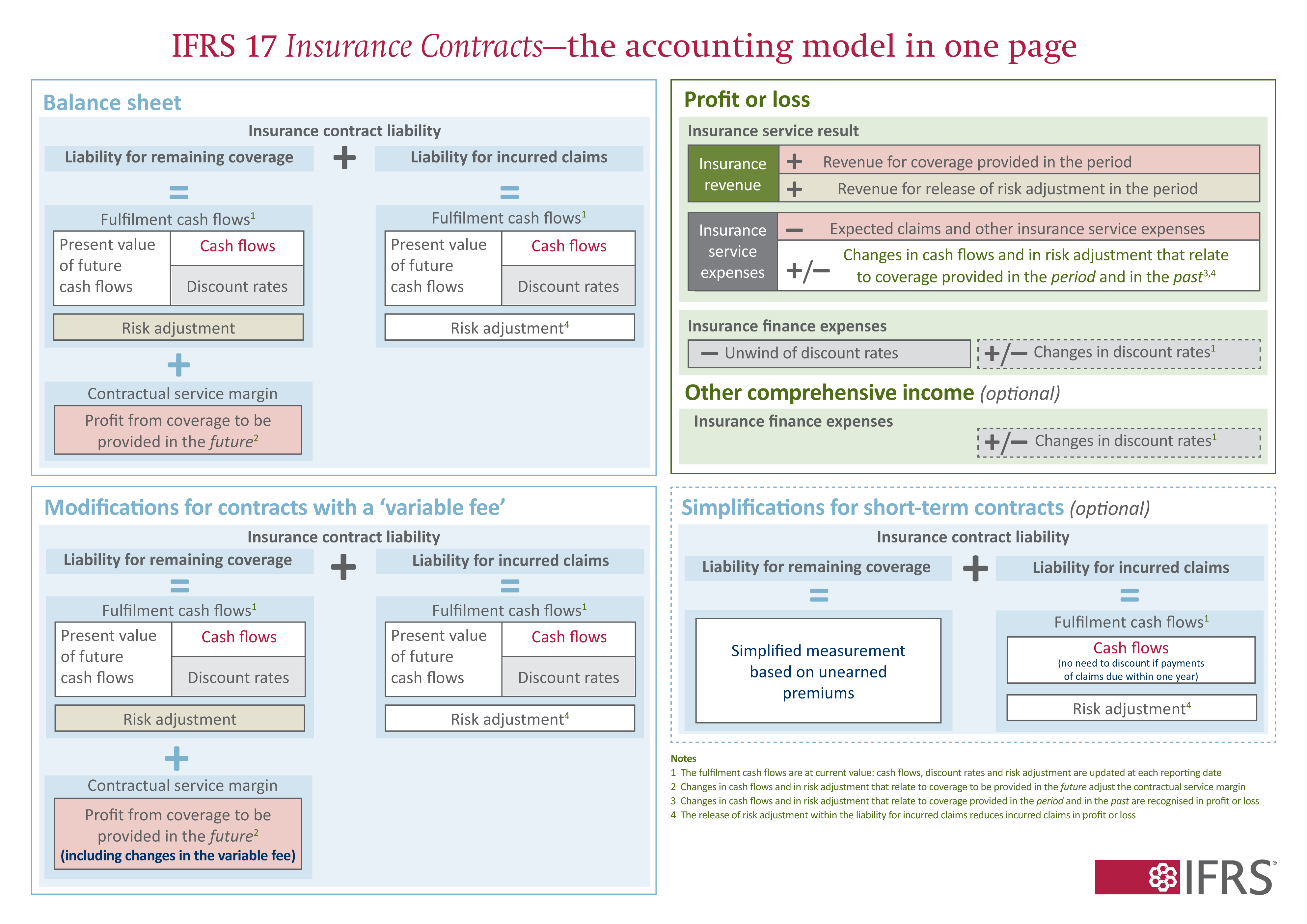
2.3.9 Simplified IFRS 17

This section describes the simplified, IFRS 17-like accounting used in our examples. Because IFRS 17 may be unfamiliar to many US readers, this description is more detailed. The original standard, International Accounting Standards Board (2017), is very clearly written and everyone should look at it at least once! Caramagno et al. (2021) provides a summary of the standard for actuaries.

The cash-flow statement is unchanged. The main difference from GAAP lies in measurement. IFRS 17 applies current-value measurement to insurance liabilities instead of the deferral-and-matching model familiar from US GAAP. GAAP defers written premium and matches it with incurred losses over time; IFRS 17 re-measures the insurer’s current fulfilment obligation each reporting date, using up-to-date cash-flow, discount, and risk assumptions.

This distinction matters most for longer-duration contracts. For one-year general insurance business the gap is narrower, and IFRS 17’s Premium Allocation Approach (PAA) largely reproduces GAAP unearned-premium accounting, but the underlying concepts differ. IFRS 17’s balance sheet is an economic valuation, not an accumulation of deferrals.

The statement of financial position (balance sheet) displays:

• Best Estimate Liability (BEL)
• Risk Adjustment (RA)
• Contractual Service Margin (CSM)
• Insurance Contract Liability (ICL = BEL + RA + CSM)
• Equity

The statement of financial performance (income statement) includes:

• Insurance service revenue
• Insurance service expense
• Insurance service result
• Net investment income (net of investment expenses)
• Insurance finance income or expense (unwind of discount and changes in discount rates)
• Operating result
• Tax
• Net income

Investment components that represent repayment of policyholder balances are excluded from revenue.

The BEL is the expected present value (EPV) of future premiums and losses. Adding the RA gives the EPV of fulfilment cash flows. The insurance contract liability is divided into the liability for remaining coverage (LRC) and the liability for incurred claims (LIC). The LIC equals the fulfilment cash flows for incurred losses. The LRC adds the CSM to ensure no profit is recognized at issue. Figure fig-ifrs-one-page provides a handy one-page summary of the IFRS 17 insurance contracts standard.

Figure 2.1: IFRS 17 on one page, source: IFRS website.

For one-year contracts, the LRC under IFRS 17 plays roughly the same role as the unearned-premium reserve (UPR) under GAAP, but with important refinements:

Table 2.2: Comparison of simplified GAAP and IFRS 17 insurance accounting.

Feature	GAAP UPR	IFRS 17 LRC
Measurement	Deferral of unearned premium	Present-value fulfilment obligation
Discounting	None	At current market rates
Risk margin	Implicit	Explicit RA component
Profit deferral	Implicit	Explicit CSM
Re-measurement	Rare	Each reporting date
Conceptual focus	Matching revenue and expense	Measuring current obligation

Thus IFRS 17’s LRC collapses back toward the GAAP UPR for short-term contracts, but conceptually it measures the insurer’s current value of remaining obligations rather than merely deferred revenue.

Example 2.1 Veith and Fieberg (2024) report that the association between stock prices and full fair value accounting items is greater than that of historical cost measurements. They compare Solvency II and an older fair value IFRS in use before IFRS 17.

Example 2.2 Solvency II and IFRS 17 share a common vocabulary—both value insurance liabilities using discounted, probability-weighted cash flows plus an explicit risk margin—but they differ in purpose and calibration. IFRS 17 measures liabilities on a fulfilment basis, representing the amount an insurer would require to settle its obligations by running them off itself. Solvency II instead adopts a transfer or exit basis: the amount a third party would demand to assume the obligations. Consequently, the risk adjustment under IFRS 17 is entity-specific, reflecting the insurer’s own risk appetite and diversification, whereas the risk margin under Solvency II is market-consistent, derived from the cost of holding capital under the standard formula or internal model until run-off. Both frameworks use current discount rates, but Solvency II prescribes market risk-free curves with an optional liquidity adjustment or matching adjustment for predictable cash flows, while IFRS 17 allows rates consistent with observable market variables that reproduce the characteristics of the liability’s cash flows. Solvency II aims at regulatory solvency and comparability across firms; IFRS 17 at faithful representation of the insurer’s economic performance. As a result, Solvency II liabilities are typically higher and more volatile, while IFRS 17 provides a smoother but more management-specific view of value creation over time.

It is helpful to think of the Contractual Service Margin (CSM) as consisting of two parts:

\[ \text{CSM} = \text{RA}_0 + \text{Service margin}, \]

where

• RA₀ is the risk adjustment at inception, corresponding to the compensation for bearing risk during the coverage period, and
• the Service margin represents the profit from providing authorized insurance service—the “paper” function—over the term. It is analogous to a fronting fee.

Together they form the unearned profit released as the insurer provides coverage and uncertainty resolves.

The Risk Adjustment (RA) shown separately on the balance sheet represents the remaining risk margin after coverage ends, associated with outstanding claims. Its release pattern is tied to the resolution of uncertainty, not the timing of cash payout. Payments may lag far behind the information that determines ultimate loss; the RA release follows the information, not the payment. This distinction—between when uncertainty resolves and when cash flows occur—is central to understanding how risk is recognized, and is a key theme of this monograph.

The fact IFRS 17 requires re-measurement each period means that discount-rate changes and updated expectations immediately affect reported profit. IFRS 17 therefore produces a balance sheet and income statement that move with economic reality, although, in our applications, the economy is fixed.

The standard also provides clear methods for determining discount rates for fulfilment cash flows (sec-discount-rate) and for presenting the unwinding of discount and rate re-measurements (sec-unwinding).

The result of twenty years’ work, IFRS 17 is a coherent, economically grounded framework: it aligns profit recognition with how insurers actually generate value—through underwriting, risk bearing, and investment skill—while transparently reflecting time value and uncertainty.

Reinsurance contracts follow the same logic but appear as reinsurance assets rather than liabilities.

2.3.10 Determining the Loss Discount Rate

US statutory and GAAP accounting both measure insurance liabilities at nominal value, disallowing any discount for the time value of money. This simplicity comes at a cost: the economic value of deferred loss payments and the embedded risk margin are obscured. The “management’s best estimate” reserving standard provides little transparency, and users cannot tell how much of the reserve represents expected loss, time value, or risk adjustment.

IFRS 17 requires discounting and also provides principled guidance for setting the discount rate—one of the most debated topics in insurance accounting. The standard requires that the rate:

reflect the time value of money, the characteristics and liquidity of the cash flows; be consistent with observable current market prices for financial instruments with similar timing, currency, and liquidity; and exclude factors that affect market prices but not the future cash flows of the insurance contracts.

Two equivalent approaches are allowed:

• Top-down: start from the yield on a broadly matched portfolio of assets and adjust downward to remove risks (credit, market) that are not present in the liabilities.
• Bottom-up: start from a risk-free yield curve and add an illiquidity premium consistent with the restricted liquidity of insurance liabilities.

The chosen rate must be disclosed and is a market rate, not entity-specific. In practice, it is slightly above the risk-free curve—risk-free with restricted liquidity—reflecting what insurers actually earn on long-dated, illiquid obligations.

Using discounted losses accelerates recognition of underwriting income, shifting part of what is traditionally treated as investment return into the measure of insurance service result. This better reflects the economics of the business, whose value arises from underwriting skill rather than investment leverage.

2.3.11 Presenting Amortization of Discount

A perennial source of confusion when discounting reserves is the unwinding of the discount. As time passes, discounted reserves accrete toward their undiscounted amount, apparently producing loss development even when expectations remain unchanged. IFRS 17 resolves this by offsetting the effect of discount unwinding not as underwriting loss but against investment income.

Specifically, it introduces an income-statement item called Insurance Finance Expense (IFE), which offsets the interest accretion on discounted reserves against investment income. Conceptually, investment income is divided into two parts:

• Insurance investment income: the portion needed to unwind the discount and maintain the discounted value of liabilities; and
• Operating investment income: the residual attributable to shareholders’ funds.

This treatment preserves underwriting income from spurious “development” while keeping the balance sheet internally consistent: reserves grow with interest, funded by the corresponding portion of investment return.

2.3.12 The Pentagon of Insurance Accounting Metrics TODO

The insurance pentagon, Figure fig-pent, displays key insurance pricing variables and the relationships between them. It was introduced in PIR Chapter 10.5. The pentagon view is for a single-period. There are five monetary variables: premium, loss, margin, assets, and capital, and three ratios describing leverage, loss ratio, and return.

Figure 2.2: The insurance pentagon

Table tbl-pentagon displays a number of relationships between the eight key insurance variables which we use repeatedly: you should become familiar with them. The table uses Greek letters for the ratios and Roman for monetary amounts.

Table 2.3: The eight pentagon variables and relationships between them and with other insurance statistics.

Ref	Variable or relationship	Interpretation
	Monetary amounts
1	\(L\)	Expected loss
2	\(P\)	Premium
3	\(M\)	Margin
4	\(a\)	Total assets
5	\(Q\)	Capital
	Related amounts
	\(a-L\)	The unfunded liability above expected loss, funded by margin and capital
	Monetary identities
Prem	\(P=L+M\)	Premium is expected loss plus margin
Fund	\(a = P + Q\)	Funding equation: premium and capital only source of \(t=0\) assets
	Ratios
6	\(\lambda = L/P\)	Loss ratio
7	\(\gamma = P/a\)	Premium to asset leverage (gamma=g for leveraGe)
8	\(\iota = M/Q\)	Expected return on capital (investor) or cost of capital (insured)
	Related ratios
	\(\nu = 1/(1+\iota)\)	Risk discount factor, analog of \(v=1/(1+i)\)
	\(\delta = \iota /(1+\iota)\)	Risk discount rate, analog of paying interest at \(t=0\)
7a	\(P/Q= \gamma/(1-\gamma)\)	Premium to capital leverage ratio, divide top/btm by \(a\), used Fund
	Ratio identities
	\(\delta = \iota \nu\)	Analog of \(d=iv\) in theory of interest
Disc	\(1 = \nu + \delta\)	Analog to \(1=v+d\)
	Capital identities
Q	\(Q=\nu(a-L)\)	\(Q\) is \(t=0\) price paid for asset with expected \(t=1\) return \(a-L\)
8a	\(\iota = (P-L) / (a-P)\)	Substitute Prem and Fund into (8)
	\(\delta = (P-L) / (a-L)\)	Substitute Prem and Fund into (8)
	Premium identities
P1	\(P=\nu L + \delta a\)	Premium \(=\) weighted average of expected loss and maximum loss, \(a\)
P2	\(P=a - \nu(a-L)\)	Premium \(=\) assets not funded by investor capital
P3	\(P=L + \delta (a-L)\)	Premium \(=\) expected loss plus share of unfunded liability
P3a	\(P=L + \iota Q\)	As P3 but expressed in terms of cost of capital

Premium, like discount, is received at \(t=0\) hence the relevance of \(\delta\). Income, like interest, is earned and paid at \(t=1\) and measured with \(\iota\). Discount is easier to work with as a measure of return because it is always between \(0\) and \(1\): \(\delta=1\) corresponds to an infinite return.

Pricing is the process of splitting the unfunded liability \(a-L\) into premium margin and capital parts funded by the policyholder and investor respectively. The risk discount factors tell you how to accomplish this.

The relationship between premium and loss can be expressed using the loss ratio or its reciprocal, the premium multiplier. The latter is sometimes used in catastrophe pricing, when loss ratios seem embarrassingly low. Likewise, leverage could be expressed as premium to capital rather than premium to assets. The point is there is a measure of leverage, a measure of margin to volume and a measure of return-cost to capital.

Given required expected return from a top down approach analysis, the standard pentagon equations in Table tbl-pentagon show that knowing \(\iota\), \(L\), and \(a\) determines total premium. It can be expressed in multiple ways, the most helpful of which are \[ P = L + \delta (a-L) = L + \iota Q = \nu L +\delta a. \tag{2.1}\] The first two expressions make it clear that premium equals expected loss plus cost of capital. The third will reappear again and again in this monograph.

2.3.13 The Pentagon with Discount and Reserves TODO

Reserves are denoted \(V\) because they are reserVes, or, following the parallel reserving to Valuation in life insurance. The letter \(R\) is used for risk adjustment release and \(\text{RA}\) for the risk adjustment liability.

2.3.14 Premium Determination versus Explaining Premium

Insurance pricing identities are implicit equations linking key accounting quantities such as premium (\(P\)), loss (\(L\)), expenses (\(E\)), and margins. Under GAAP, the familiar expression \[P = L + E + \text{UW Margin}\] and under IFRS 17, its analogue \[P = \text{PV(Loss)} + \text{RA} + \text{CSM}\] can each be written more abstractly as \[f(P, L, E, \text{RA}, \text{CSM}, \ldots) = 0\] for some pricing function \(f\). This form highlights that “pricing” is not a single operation but the solution of an implicit functional relation. Depending on which variable we solve for, the same identity serves different purposes.

Premium determination treats \(P\) as the unknown. It solves the accounting identity for the premium required to meet a target return, given expected losses, expenses, and capital costs. This is the familiar forward use of the pricing equation: find the price that balances the books under the chosen accounting view.

Premium explanation takes \(P\) as given and solves instead for another variable—often the implicit underwriting margin, risk adjustment, or service margin—that reconciles the observed premium with modeled losses and expenses. It is the inverse problem: explaining how a market or booked price decomposes across the accounting components of the chosen framework.

These are two sides of the same implicit-function relation. Accounting standards determine which variable appears explicit and which implicit, but the underlying economic relation is invariant. A GAAP statement and an IFRS 17 statement describing the same contract are different parameterizations of the same surface in \((P,L,E,\text{RA},\text{CSM})\) space. The ability to move between these views—solving for \(P\) or explaining it—is what allows consistent interpretation of pricing results across accounting regimes.

2.4 Contracts with Contingent Cash Flows

contract template · cash flow vector · sign convention (loss/payoff) · position (long/short) · market structure and role · bid and ask prices · placement (asset/liability) · function · information · cat bonds

2.4.1 Introduction

A contract with contingent cash flows (a CCF contract) is a formal agreement defining the transfer of value between two parties—traditionally labeled the Long and the Short—based on future events. A CCF contract has cash flows that depend on future states of the world, but it does not presume tradability, regulatory treatment, balance-sheet placement, or market micro-structure. This terminology keeps the focus on economics rather than institutional classification and allows insurance, reinsurance, and financial contracts to be analyzed within a single, consistent framework.

Terminology varies across markets. I reuse familiar words (Long, Short, bid, ask, dealer, broker) in a deliberately abstract way to unify notation across settings; when a market uses these terms more narrowly, treat the mapping as approximate and follow the definitions given here.

Remark 2.2 (Why “CCF contract” instead of “security” or “asset”). We prefer CCF contract to security because security is heavily overloaded. In legal and regulatory contexts it has a precise meaning defined by bodies such as the Securities and Exchange Commission, while in market practice it often connotes tradable financial instruments governed by securities law. That meaning is subtly but importantly different from commodity-style contracts regulated by exchanges such as the Chicago Mercantile Exchange, and different again from insurance contracts, which sit outside both regimes. Using security as a generic label therefore risks importing unintended legal, regulatory, or market connotations. Another alternative is asset, but the same CCF contract can be an asset or a liability. To avoid these ambiguities, we adopt the neutral term contract with contingent cash flows.

Remark 2.3 (Primary and derivative contracts). Traditional accounting distinguishes between “primary” securities and “derivatives,” but a rigorous contingent-claims view reveals that almost all financial instruments are contingent claims. As Robert Merton demonstrated in 1974, even the capital structure of a firm fits this lens: equity resembles a long call option on the firm’s assets, while a corporate bond resembles a long position in a risk-free asset combined with a short put option granted to shareholders. From this perspective, the distinction between a stock, a bond, and a credit default swap is not one of kind, but of the specific triggers and topologies of the underlying contingencies.

2.4.2 The Contract as a Template

A CCF contract starts as a template with blank spaces for the parties’ names, a schedule of contingencies, and an up-front transaction cash flow (the price paid by one side to enter the contract). The contingencies define state-contingent cash-flow magnitudes and directions: “If event \(i\) occurs, the Short pays the Long amount \(A_i>0\),” or the reverse. In this framework, each payment has a positive magnitude (the amount \(A_i\)) and a direction (Long to Short, or Short to Long). Which party experiences which cash flows depends on which role they occupy.

A CCF contract normally includes several standard clauses.

1. The named Parties to the transaction. CCFs are usually bilateral.
2. Effective and expiration Dates, important to specify the contract boundary.
3. The Trigger Event: the stochastic state variable (e.g., total losses from insured events, a hurricane’s landfall intensity, or a stock’s closing price).
4. The Payoff Function: the mathematical rule determining the cash-flow amount from the state variable.
5. The Settlement Method: whether the contract is settled via physical delivery or cash.
6. The Calculation Agent: the “oracle” responsible for determining the terminal value.
7. Any Cash Due at Inception, representing the “price” or “premium”.

As the contract is negotiated each of these is gradually filled in. For exchange traded contracts the clauses are very standard. In negotiated markets such as reinsurance the wording of the contract is itself subject to negotiation.

2.4.3 Cash Flow Vectors and Loss vs. Payoff Sign Conventions

In a CCF contract, we treat a cash flow as a vector, or directed quantity, not a signed scalar. Like velocity, it has a non-negative magnitude, called its amount, and a direction: either “Long to Short” or “Short to Long.” (Amount is analogous to speed, and direction to bearing.)

When we collapse a CCF cash-flow vector to a signed scalar quantity we need a sign convention.

Definition 2.1 (Cash flow scalar sign conventions.)  

• The loss sign convention models payments made as positive
• The payoff sign convention models payments received as positive

Under the loss convention, the right tail is bad: higher values mean larger outflows. It is used for insurance losses. We usually use \(X\) for variables using the loss convention. Under the payoff, the left tail is bad: lower values mean greater amounts owed. We usually use \(Y\) for variables using the payoff convention.

The sign convention is a modeling choice and not part of the contract. The contract specifies the cash-flow vector explicitly; the sign convention enters only when the cash-flow vector is mapped into a signed random variable \(X\) representing one participant’s perspective. To specify \(X\), we must specify the perspective (Long’s or Short’s) and the sign convention.

1. For a fixed sign convention, negating \(X\) switches perspective: if \(X\) is defined from Long’s perspective, then \(-X\) is defined from Short’s perspective, and vice versa.
2. For a fixed perspective, negating switches sign conventions: Long-payoff \(X\) becomes Long-loss \(-X\), and Short-payoff \(X\) becomes Short-loss \(-X\).
3. Combining bullets 1 and 2, the same value of \(X\) can be read as Long-payoff and Short-loss, or as Long-loss and Short-payoff.

Table tbl-four-signs shows the signed cash flow corresponding to the cash flow vector “Short pays Long \(1\)” under each perspective and sign convention.

Table 2.4: The same cash flow by sign-convention and perspective.

Item	Long's perspective	Short's perspective
Payoff sign-convention	+1	-1
Loss sign-convention	-1	+1

Insurance cash flows are commonly modeled with the payoff convention from the insured’s (Long) perspective and the loss convention from the insurer’s (Short) perspective. The Long/payoff and Short/loss views coincide because of the double negative \((-1)(-1)=1\).

Remark 2.4 (Vector space interpretation of cash flows). Cash flows are a vector in a one-dimensional real vector space. We can pick as basis \(\mathbf{1}_{A\rightarrow B}\) or \(\mathbf{1}_{B\rightarrow A}\) denoting, respectively, a payment of amount \(1\) from \(A\) to \(B\) or \(B\) to \(A\). Then, the table shows the slight ambiguity: the four expressions \[ -\mathbf{1}_{A\rightarrow B} =(-1)\mathbf{1}_{A\rightarrow B} =(+1)\mathbf{1}_{B\rightarrow A} =\mathbf{1}_{B\rightarrow A} \] all represent the same cash flow, c.f., Table tbl-four-signs. Both are equal and also equal to $$. Picking the basis corresponds to selecting the sign convention. The scalar in a vector space can be positive or negative, whereas we consider the magnitude of a cash flow to be positive. Requiring positive cash flows in this way allow contracts to be written unambiguously without specifying a basis.

2.4.4 Contingent Cash Flows

Definition 2.2 A contingent cash flow is a stochastic process specifying nominal monetary cash flows, in a specified unit of account, at future times, contingent on future states of the world. A single-payment contingent cash flow is a random variable giving the cash flow at a single future time.

The definition is deliberately broad. In some academic settings there is a single consumption good used as the unit of account; here the unit of account is the contract’s currency, but the same abstraction applies.

Example 2.3 (CCF Contracts.) Here are standard examples of contracts and their underlying contingent cash flows.

1. A stock; cash flows: dividend payments and any residual (liquidation) value.
2. A bond; cash flows: coupon payments and return of principal.
3. A stock or index forward (or future, which is an exchange-traded forward with daily settlement); cash flow at maturity (ignoring interim margining): \(S_T - F_0\) per share (or per contract share multiplier), where \(S_T\) is the stock or index price at \(T\), and \(F_0\) is the delivery price set at inception.
4. A stock option. European call: payoff at maturity: \(\max(S_T - K, 0)\) per share (or contract multiplier). European put: payoff at maturity: \(\max(K - S_T, 0)\) per share (or contract multiplier). American options allow exercise at any time before expiration.
5. A weather derivative; payoff: a function of the number of heating or cooling degree days, or the cumulative number of degree days the temperature is above or below a strike over the contract period.
6. A property insurance policy; payoff: a function of the individual and aggregate loss after applying occurrence and aggregate limits and deductibles.
7. An aggregate excess of loss reinsurance contract; payoff: aggregate losses from an underlying book subject to a retention and aggregate limit.

2.4.5 Position: Long or Short

Any contract has two sides, and we must specify which side the model represents in order to determine actual cash flows. For historical reasons the two sides are called the Long and the Short. Broadly, the long party tends to:

• benefit from an increase in the value of the underlying,
• own the claim,
• pay when the contract is entered into (in many, but not all, settings), and
• take delivery or receive the asset (when settlement is physical).

The short party has the opposite characteristics: they owe or write the claim, often receive cash at inception, and deliver the asset (or make the payment) under the contract’s triggers. A cash flow for the short position is always the vector negative (opposite direction) of that for the long.

Example 2.4 (Long and short sides of standard contracts.)  

• For an insurance contract, the insured takes the long position, giving them the right to indemnity payments contingent on loss. The insurer takes the short position, writing the contract. The loss is the underlying; it may be transformed by policy limits and deductibles.
• For a reinsurance contract, the insurer takes the long position and the reinsurer the short.
• For an option, the long position buys the option, giving them the right, but not the obligation, to transact at a specified strike. The short position sells (writes) the option and must perform if exercised. (For a put, the long benefits from a decrease in the underlying, not an increase.)
• For a future or forward, the long position agrees to buy the underlying asset on a specified future date for a specified price, and the short position agrees to deliver. There is typically no initial transaction when these contracts are entered into. In this case, both parties have obligations at expiration so neither strictly “owns the claim.”

Remark 2.5 (Parties, positions, and the language of “owning”). It is useful to distinguish parties to a contract from the colloquial ideas of owning, buying, or selling a contract. Strictly speaking, contracts are not owned; they are entered into. A contract is a legal relationship between counterparties that specifies reciprocal rights and obligations, and those rights and obligations exist only by virtue of the parties’ participation. The language of ownership arises once contracts become sufficiently standardized and transferable that the economic exposure can be separated from the original counterparty relationship. Exchange-traded futures and options are the canonical example. For bespoke insurance and reinsurance contracts, by contrast, “ownership” is misleading: the contract exists only between named parties, cannot be freely transferred, and is better described in terms of who is bound by it.

Remark 2.6 (The Origin of Long and Short). This terminology originates from the use of tally sticks in medieval Europe, particularly in the English Exchequer. When two parties entered an agreement—such as a loan or a contract to deliver goods—they would record the details on a hazel wood stick.

• The Long Side (the Stock): The stick was split down the middle, but not perfectly. One piece was kept longer than the other. The longer piece, called the “stock” (hence the term “owning stock”), was given to the party who had the claim or was “owed” the asset. This person was “long.”
• The Short Side (the Foil): The shorter piece, called the “foil,” was given to the party who had the obligation to deliver the asset or repay the debt. This person was “short.”

The term “short” has roots in common English usage dating back to the mid-19th century (and likely earlier in merchant circles). To be “short” simply means to be “lacking” or “in deficit” of something (e.g., “I am short of cash”). In a futures or forward contract, the seller is “short” the commodity because they have committed to delivering something they may not yet physically possess. They are in a state of deficiency relative to their contractual obligation.

The beauty of the tally system is its biometric security: because hazel wood grain is unique and the split follows the natural fibers, the “Short” piece (Foil) would only fit perfectly back into the “Long” piece (Stock) if they were the original pair. This made the “Short” side’s obligation and the “Long” side’s claim verifiable and tamper-proof.

2.4.6 Market Structure and Market Roles

Transactions involving CCF contracts occur within three primary market structures:

1. Quote-driven (dealer) markets: intermediaries (market makers) provide continuous liquidity by standing ready to take either side of the contract.
2. Order-driven (auction) markets: a centralized system matches buyers and sellers directly based on price and time priority.
3. Brokered (negotiated) markets: brokers facilitate bespoke matches between specific parties who often have predetermined roles.

Participants in a market have different roles and it is useful to distinguish three:

1. Solicitor (searcher): initiates contact and begins counterparty search.
2. Quoting party (maker, liquidity provider or supplier): names a firm, executable price for a specified oriented contract.
3. Accepting party (taker, liquidity demander): accepts a firm quote and executes immediately at the maker’s terms.

Solicitation and quote-taking are independent. A party can solicit and still end up quoting, or solicit and end up taking, depending on who supplies terms and who accepts them.

A quote is firm in the limited but essential sense used here: conditional on any stated assumptions, it is a price at which the quoter stands ready to trade immediately if the other party accepts. (Indicative quotes do not define bid/ask until converted into firm terms.)

2.4.7 Bid and Ask Prices

In the benchmark model of asset pricing, markets are competitive and trading is unconstrained. Prices are then well described by a single linear pricing rule: a functional that assigns a unique price to each cash-flow process and respects additivity and scaling. In that setting, no-arbitrage is powerful, and—together with replication in a complete market—it implies exact equalities such as the Black–Scholes option pricing formula.

In the classic frictionless market, trading is costless (no transaction costs), assets are perfectly divisible, and no agent has market power. Prices satisfy the law of one price: two securities with the same future cash flows have the same current price. This produces a single pricing functional \(p(\cdot)\) that is linear:

• \(p(X+Y)=p(X)+p(Y)\),
• \(p(kX)=kp(X)\) for all \(k\) (not just \(k>0\)),
• \(p(c)=c\) for sure cash \(c\) (or \(p(c)=\beta c\) if you separate discounting),

The risk-neutral measure representation that actuaries meet in finance texts is one convenient way to express this linear functional, but linearity is the key point for what follows.

Real markets depart from that textbook benchmark. Trading can be costly, constrained, or capital intensive. Common frictions include transaction costs, inventory and funding costs, margin and collateral requirements, information asymmetry, position limits, short-sale constraints, and costly capital. Once these frictions matter, it is natural to model two prices, the bid and ask defined as follows.

Definition 2.3 (Bid and Ask Prices) For a given contract, which fixes the obligations of the long and short sides:

• The ask is the amount paid at inception when the long side is the taker (it accepts the short side’s quote).
• The bid is the amount paid at inception when the long side is the maker (its quote is accepted by the short side).

Typically, the ask is paid by the long and the bid by the short, and the ask exceeds bid. The bid-ask spread or simply spread is the ask minus the bid. The spread is borne by the liquidity demander: the demander receives a less favorable price than it would receive if it were supplying liquidity. The spread is not an arbitrage by itself, because round-tripping is no longer free. The actual direction of cash flow depends on the specifics of the contract because amounts are always positive!

The bid-ask spread is the cost of immediate execution. Its determinants include order-processing and operating costs, inventory and funding costs borne by the liquidity supplier, and adverse-selection costs arising from asymmetric information.

Spreads are ubiquitous. Results from Bellini et al. (2020) imply that SRMs add a non-zero spread to all non-constant risks. If there is a single non-constant risk with no spread then the SRM is just a multiple of the mean, or it “collapses to the mean”.

TL;DR: When you accept a firm quote, you pay the spread.

The bid–ask spread is not just a detail of quoting. It signals a change in market structure. With frictions, prices become nonlinear and “no-arbitrage” becomes a family of conditions. Pricing functionals are typically monotone and cash-invariant, but not linear. Under nonlinear pricing, there are several non-equivalent “no-arbitrage” concepts depending on the transactions needed to create potential arbitrages. One approach is to demand the absence of buy and sell arbitrage opportunities, see Chateauneuf and Cornet (2022) and Bastianello et al. (2024).

In a quote-driven market, the market maker faces directional uncertainty. When a customer approaches, the dealer does not know whether the customer intends to be the long or the short. To manage this, the dealer provides a two-sided quote on the up-front transaction price. The customer pays the ask to enter as long and receives the bid to enter as short. The spread compensates the dealer for inventory risk, funding and operating costs, and uncertainty about which side the customer will take, including adverse-selection risk.

In brokered (negotiated) markets—such as the reinsurance “Firm Order Terms” or “Best and Final Quotes” process—identities and roles are typically fixed from the outset. A seller knows they are selling, and a buyer knows they are buying. Negotiation proceeds through iterative, one-sided quotes toward a single agreed price. In the last instance, one party accepts the other’s final firm terms. Relative to a fixed oriented contract, either (i) the long side accepts the short side’s final quote (execution at the ask), or (ii) the short side accepts the long side’s final quote (execution at the bid).

In reinsurance, the long side’s final firm quote is often called a firm order term. In a hard market, the firm order term commonly matches the reinsurer’s quoted terms, so execution occurs at the reinsurer’s ask for \(X\). In a soft market, the firm order term can lie below the reinsurer’s most recent quote; if the reinsurer accepts it, execution occurs at the bid for \(X\).

Small commercial and personal lines insurance behaves like a quoted market in the present sense that insurers commonly supply terms and insureds commonly accept them. Large commercial insurance and reinsurance behave like negotiated markets: solicitation and bargaining are central, and executable terms emerge only after an exchange of quotes and counterquotes.

Remark 2.7 (Valuation acquire/dispose interpretation of bid and ask prices). Definition def-040-bid-ask-01 defines bid and ask using the maker/taker, market micro-structure perspective. In terms of cost to acquire or dispose of a position in a contract, this is phrased as:

• The ask is the amount required to acquire the long position in the contract.
• The bid is the amount received to dispose of the long position in the contract.

The two definitions are consistent as they describe the same economic cash flows for a participant seeking or holding a long position.

Table 2.5: sdaf

Term	Taker/Maker Perspective	Cash Flow Perspective	Logical Link
Ask	Long side is the taker. They pay the price set by the seller.	Amount required to acquire the long position \(X\).	To acquire a position as a taker, one pays the higher price (the Ask).
Bid	Long side is the maker. Their quote is accepted by the short side.	Amount received to dispose of the long position \(X\).	To dispose of a position, one receives the price the market is willing to pay (the Bid).

There is an important relationship between bid and ask prices.

If a single dealer (or a single internally consistent pricing rule) quotes prices for both \(X\) and \(-X\), then “acquiring \(X\)” is the reverse trade of “disposing of \(-X\).” When those two descriptions refer to the same economic trade against the same quotes, the prices must match up to sign. That assumption enforces an important relationship between bid and ask prices.

Proposition 2.1 (Bid-Ask Pricing Relationship) Assume bid and ask quotes come from a single internally consistent quoting rule applied to both \(X\) and \(-X\), with no counterparty credit risk. Then \[ \mathrm{ask}(X)=-\mathrm{bid}(-X). \tag{2.2}\]

Proof. Buying the security with long position \(X\) requires an upfront outflow of \(\mathrm{ask}(X)\) and produces the future cash flow \(X\). Selling (disposing of) the security with long position \(-X\) produces an upfront inflow of \(\mathrm{bid}(-X)\) and leaves the seller obligated to pay \(-X\) in the future, which is the same as receiving \(X\).

Thus, buying \(X\) and selling \(-X\) create the same future cash flow \(X\) against the same quoting rule. With no counterparty credit risk, internal consistency requires their upfront cash flows to match up to sign: \[ -\mathrm{ask}(X)+\mathrm{bid}(-X)=0, \] which implies \(\mathrm{ask}(X)=-\mathrm{bid}(-X)\).

This proposition does not depend on a loss vs payoff sign convention. It follows from reversing the position.

Example 2.5 The framework applies to the securitization of insurance losses. Let the random variable \(X\) represent losses on an insurance policy with a maximum loss \(a\). When an insurer writes the policy \(X\) backed by assets \(a\), they become short \(X\) and the insured is long. The insured pays \(\mathrm{ask}(X)\) to initiate their long position. At this point, the insurer is long the residual payoff \(Y := a - X\). It can exit its position for \(\mathsf{bid}(a-X)\), leaving it obligated to pay \(a\) in every state. The investor becomes long \(a-X\). By no arbitrage, \[ \mathrm{ask}(X)+\mathrm{bid}(a-X)=a. \] But, \(\mathrm{bid}(a-X)=a+\mathrm{bid}(-X)\) and so \(\mathrm{ask}(X)=-\mathrm{bid}(-X)\). \(\quad\square\)

Frictionless markets, with linear pricing rules, do not have a spread because the bid equals the ask: \(-p(-X)=--p(X)=p(X)\). Notice that if \(p\) is just positive homogeneous this doesn’t work: it relies on applying homogeneity with constant \(-1\).

The literature suggests many reasons why a market might include a spread: information asymmetry, inventory risk, operating costs, and funding and margin costs. For insurance and reinsurance, two additional forces matter repeatedly.

1. Costly capital and limited risk-bearing capacity. Holding risk consumes scarce capital, and capital has a required return. This creates wedges between expected value and transaction price, and it becomes more severe for concentrated, illiquid, or tail-heavy risks. Froot develops this idea for insurers and reinsurers, building on Froot and Stein’s capital allocation framework (Froot 2007; Froot and Stein 1998).

2. Default or performance aversion. Many insurance customers care about the insurer’s ability to perform in bad states. That preference makes “risk transfer” different from a pure expected value trade, and it supports nonlinearity and spreads even when the nominal contract looks simple (Froot 2007).

In catastrophe reinsurance and other opaque, nonstandard risks, intermediation itself becomes part of the product: intermediaries specialize in bearing and managing these risks, but they do so at a cost that shows up as a spread over “fair” value (Froot and O’Connell 2008).

Remark 2.8 (Related literature). The connection between limited loss and residual \[ a = (X\wedge a) + (a - X)^+ \] is reminiscent of put-call parity. Put-call parity has two subtly different formulations. Writing \[ X - a = (X-a)^+ - (a-X)^+ \] leads to a Put-Call Partity (PCP) condition for a translation invariant pricing functional \(f\) that requires \[ f(X) - a = f(X-a)^+ + f(-(a-X)^+). \] We can also write \[ (a-X)^+ = (X-a)^+ - X + a \] leading to a Call-Put Partity (CPP) condition \[ f((a-X)^+) = f(X-a)^+ +f(-X) + a. \] The fact that \((X-a)^+\) and \(-(a-X)^+\) are comonotonic, whereas \((X-a)^+\) and \(-X\) are not is an important difference between these formulations. Cerreia-Vioglio et al. (2015) shows that \(f\) satisfies PCP, translation invariance and monotonicity if and only it it is a Choquet pricing rule. A SRM is a subadditive Choquet rule. Notice this implies law invariance and comonotonic additivity. Bastianello et al. (2024) shows that if \(f\) is monotone then is satisfies CPP if and only if it has a formulation as a Choquet-Šipoš pricing rule—a slightly different formulation of the Choquet integral that treats upside and downside symmetrically. See also Chateauneuf and Cornet (2022). \(\quad\square\)

To conclude: bid–ask spreads are not a defect of the model. They are the model’s way of admitting that trading risk is costly, capital is scarce, and different agents face different constraints. Under mild regularity, imposing law invariance together with too much linearity forces a pricing functional to reduce to (an affine transform of) expectation, so non-trivial pricing requires genuine nonlinearity (Bellini et al. 2021).

2.4.8 Accounting Placement: Asset or Liability

The same CCF contract can be an asset or a liability, reported on the left or right of the balance sheet. A CCF is held as an asset when the present value of its expected rights to receive cash exceeds the present value of its expected obligations to pay, and otherwise it is held as a liability. A contract’s name does not determine placement; expected rights and obligations determine placement.

A security can be issued as a liability but later become an asset. For example, consider a very profitable, low-risk insurance policy. If the premium is paid in advance it is a liability (only loss payments remain). If premium is deferred it can be an asset because the insurer has a premium receivable that dominates expected loss payments.

Under IFRS 17, groups of insurance contracts issued and reinsurance contracts held each present as either an insurance contract asset or liability depending on net fulfilment cash flows at the reporting date. An insurance CCF corresponds to contracts typically issued as a liability, but that can net to an insurance contract asset when rights to cash exceed obligations (e.g., front-loaded premiums or the insurance acquisition cash flow asset that IFRS 17 carries and then recoups from future premiums). A reinsurance contract held is usually a liability when issued, because it contains a positive margin for the reinsurer, but it may become an asset depending on covered losses. The IFRS 17 treatment depends on the prior grouping of contracts into onerous and non-onerous.

2.4.9 Contract Function

Actuaries are expected to be familiar with insurers’ financial statements, which are atypical because insurance contracts dominate the right-hand side of the balance sheet. To gain a broader understanding, it helps to compare financials for a manufacturer, a bank, and an insurer.

A manufacturer’s balance sheet centers on operations. Its key contracts support producing and selling goods: trade credit, customer advances, leases, and occasional borrowing. The operating cycle converts cash to inventory to receivables back to cash, servicing these claims and creating profit. Financial instruments appear, but production assets and working capital dominate. Hedging instruments may be used to reduce cost volatility for important inputs.

Banks and insurers look different because their businesses are financial intermediation and risk transfer. Their assets are mostly financial (loans and securities for banks; bond-heavy portfolios and reinsurance recoverables for insurers). Each issues a distinctive kind of CCF contract. Banks accept deposits—claims designed to function as money and liquidity. Insurers issue insurance contracts—contingent claims designed to transfer risk and fund uncertain, often long-dated obligations. A bank earns the spread between its funding costs and the yield on its assets, plus fees. An insurer earns underwriting margin and investment income while transforming premium funding into claim payments over time. In both, the core business is managing risk, timing, and spread.

CCF contracts have six functions by economic purpose, independent of whether they appear as assets or liabilities:

1. Operating. Arising from producing and delivering goods and services: trade credit (receivables/payables), accrued expenses, customer advances, deferred revenue, warranty obligations, taxes payable, leases tied to operations, and similar working-capital and operating-cycle claims.
2. Investment. Held primarily for income, capital appreciation, or liquidity: cash, government and corporate bonds, loans, equities, mutual funds and ETFs, repos, securitizations, and collateral arrangements.
3. Financing. Raise capital or funding and include equity and debt issues.
4. Deposit. Claims designed to provide transaction and liquidity services: bank deposits (and close substitutes), typically redeemable at par on demand or short notice. Deposits are concentrated in banks, though some non-banks issue limited deposit-like claims (e.g., gift cards or store credit).
5. Insurance. Contingent claims that transfer non-financial risk: insurance policies and reinsurance contracts. Insurance uses its own terminology: these contracts are usually called policies or contracts and they are written or issued rather than sold. Insurance-like liabilities outside insurance exist (notably warranties), but insurance contracts are concentrated overwhelmingly in insurers and reinsurers.
6. Hedging. Contingent claims used to offset or mitigate existing economic and financial exposures: derivatives, swaps, and other specialized contracts. While many CCFs can serve a hedging function, one is specifically a hedge when its primary purpose is to reduce the volatility of an existing portfolio. Hedging is often characterized by an “initiator’s premium,” where a party accepts a less favorable price to achieve immediate and certain risk reduction.

Insurance and reinsurance can be analyzed using financing concepts because they embed funding and timing transformation, but we classify them as insurance contracts because risk transfer is their primary economic purpose.

2.4.10 Asymmetric Information, Model Transformation Risk, and Structural Frictions

The complexity of CCF contracts is compounded by the nature of their contingencies. In many exchange-traded markets—stocks, rates, and widely traded commodities—the object being traded is standardized, prices are public, and value is disciplined by continuous trading and rapid feedback. Private information still exists, but it is diluted by disclosure rules, deep liquidity, and fast price discovery.

Insurance markets sit closer to the canonical “second-hand car” problem. The contract’s cash flows are tightly linked to characteristics that are privately observed (or costly to verify) and to actions taken after the contract is written. As a result, a CCF contract can embed two distinct uncertainties: type uncertainty (hidden risk or quality at inception) and action uncertainty (hidden behavior after inception). When cash flows depend on private information or behavior, the market faces asymmetric-information risks:

• Adverse selection: high-risk parties are more likely to seek the contract (the lemons problem).
• Moral hazard: possession of the contract alters behavior, increasing the probability or severity of a payout.
• Signaling: the better-informed party takes a costly action to credibly convey information.
• Screening: the less-informed party offers a menu of choices to induce self-selection (e.g., high-deductible vs low-deductible options).

A critical asymmetry arises from model transformation risk: the risk created when a qualitative written description is collapsed into a quantitative pricing model. In insurance, the insured “owns” the underlying risk and often has a more intuitive, if not statistical, understanding of it. The insurer bears the primary burden of parameter risk—the danger that the model used to represent the contract’s contingencies is miscalibrated or misspecified. While the insured evaluates the premium’s utility, the insurer faces the existential risk that the contract’s “if-then” logic triggers cash flows at a frequency or severity the model fails to predict.

Finally, these contracts are subject to three structural frictions:

• Basis risk: the gap between the actual loss suffered and the payout triggered by the contract’s language.
• Credit (counterparty) risk: the risk that promised payments are defaulted. In organized exchanges this is mitigated by clearinghouses and margin; in negotiated markets it remains a central pricing factor.
• Liquidity (exit) risk: the ease with which a party can exit their role in the contract. In fungible, quote-driven markets, a position can often be offset quickly; in negotiated, bespoke contracts, exit may require novation or commutation, and a party may be effectively locked in for the duration.

2.4.11 Capstone Example: Catastrophe Bonds

This example illustrates how a catastrophe bond transforms a (re)insurance liability into an investment security.

A catastrophe bond is a securitized instrument that bridges the insurance and capital markets using a special purpose vehicle (SPV). The structure functions through two simultaneous transactions:

1. The reinsurance leg: the SPV acts as the provider (short side) of a reinsurance contract to a sponsor insurer (long side). The sponsor pays premiums to the SPV to cover losses from a specific peril.
2. The investment leg: to collateralize its reinsurance promise, the SPV issues (short side) bonds to investors. The reinsurance premium is passed to investors as coupon payments.

The SPV passes the residual value of the bond back to the investor. If no catastrophe occurs, the investor receives the full principal; if a catastrophe occurs, the investor’s principal is reduced by the loss payment made to the sponsor. The principal usually acts as the aggregate limit of the bond so the sponsor bears no credit risk.

By passing the insurance premium to investors as a coupon spread above the risk-free rate, the SPV converts an insurance-protection position into an investment return stream. The investor becomes the ultimate provider of the insurance contingency, incentivized by a yield that compensates them for providing protection to the sponsor.

2.5 Default and Equal Priority

2.5.1 Default and Insolvency

The legal mechanics of default and insolvency illuminate the liabilities and capital hierarchy described in Section REF on Capital Structure.

Regulation typically allows a struggling insurer to enter conservation or rehabilitation, during which it is placed under regulatory supervision while attempting to restore solvency. If these efforts fail, the company is placed into liquidation.

In liquidation, assets and liabilities are handled separately, to maximize the value of assets and ensure an orderly discharge of obligations. Liquidation is managed by a receiver. All policies are canceled, and the receiver sets a fixing date, the deadline for filing claims. Pledged or collateralized assets are separated, and claims against the remaining assets are sorted into classes of priority (the pecking order) that are paid sequentially in a waterfall. Within each class, all claimants share equally.

The exact priority table is established by statute. In the United States it varies by state (see summary of priority rules by state). In some states unearned premium has the same priority as insurance claims. Claimants senior to subordinated debt are often called general creditors. Statutes uniformly give insured-loss claims high priority—both first-party and third-party liabilities arising under the insurer’s policies. Given two classes, the one paid first is senior and the one paid later is subordinated. Because administrative expenses are usually small, insurance claims are effectively the most senior liabilities.

2.5.2 Loss Payments in Default

Marginal cost depends on the exact cash flows to each unit in each possible outcome so we must specify it. So far we have ignored default and its impact on insured losses. Here we explain the mechanics of loss payments under default.

The amount paid to any unit depends on available assets \(a\), that unit’s promised loss \(X_i\), and total losses \(X = \sum_i X_i\). Dependence on the total \(X\) is critical: it couples all policies, making insurance pricing inherently portfolio-dependent.

Assume loss payments have the highest priority and the insurer has limited liability with total available assets \(a\). Promised payments \(X_i\) are limited by contract terms but not by the insurer’s assets. Aggregate losses then decompose as \[ \begin{aligned} X &= (\text{total payments}) + (\text{limited liability default}) \\ &= X \wedge a + (X - a)^+ . \end{aligned} \]

Actual aggregate payments \(X \wedge a\) must be allocated among units, which requires a default rule. The standard assumption is equal priority: all claims share proportionally in any shortfall. For unit \(i\), \[ \begin{aligned} X_i &= (\text{payment to unit } i) + (\text{default borne by unit } i) \\ &= X_i \frac{X \wedge a}{X} + X_i \frac{(X - a)^+}{X}. \end{aligned} \] Hence payments to unit \(i\) are \[ \begin{aligned} X_i(a) &= X_i \frac{X \wedge a}{X} \\ &= \frac{X_i}{X},(X \wedge a) \\ &= \begin{cases} X_i & X \le a, \\ X_i \dfrac{a}{X} & X > a . \end{cases} \end{aligned} \] Each expression shows the same relationship:

1. Payments are a constant pro-rata factor \((X \wedge a)/X\) of the contractual promise \(X_i\). The factor is the same for all units, defining equal priority.
2. Equivalently, each unit receives its share \(X_i/X\) of the assets available for loss payment, \(X \wedge a\).
3. When total losses do not exceed assets, all units are paid in full; otherwise, payments are reduced uniformly by \(a/X\).

These payments are legally determined through the receiver’s process. We refer to this as ex post equal priority, meaning that the loss shares are fixed after all claims are known.

2.6 Modeling Volatility

This section summarizes how actuaries model loss volatility and explains how publicly available industry data can be used to calibrate it. The goal is not to teach stochastic modeling but to align on conventions for representing uncertainty in ultimate loss.

Volatility modeling sits at the intersection of data, judgment, and structure. At the macro level, the industry parameters ensure consistency across lines. At the micro level, the frequency–severity and mixing frameworks determine how uncertainty propagates through the portfolio. These components together define the ultimate loss distribution—the central object of all subsequent valuation, risk, and pricing analyses.

2.6.1 Frequency–Severity Framework

Actuarial loss models start with the decomposition \[ X = \sum_{j=1}^{N} Y_j, \] where \(N\) is the number of claims and \(Y_j\) their individual severities. Conditional on \(N=n\), the \(Y_j\) are assumed i.i.d. with mean \(m_Y\) and variance \(s_Y^2\). The aggregate loss \(X\) therefore has \[ \mathsf P(X) = \mathsf P(N),\mathsf P(Y), \qquad \mathsf{var}(X) = \mathsf P(N)s_Y^2 + s_N^2 m_Y^2. \] This compound model (often compound Poisson) captures the two natural sources of volatility: claim count and claim size. Extensions introduce dependence through shared mixing variables or hierarchical structures—e.g., a random intensity \(\Lambda\) in a mixed Poisson model, \(N|\Lambda \sim \text{Poisson}(\Lambda)\). The distribution of \(\Lambda\) captures parameter uncertainty, exposure heterogeneity, and latent environmental effects such as inflation or weather.

2.6.2 Mixing and Stratification

Shared mixing variables provide a flexible way to model common drivers of loss. A single \(\Lambda\) shared across policies represents portfolio-wide shocks; stratified \(\Lambda_k\) by business segment or payout type allow for partial correlation within groups. The same technique can be used to stratify by payout year. This is the standard tool actuaries use to reflect correlated frequency or severity components without imposing explicit copulas.

A simple example is the mixed Poisson or Poisson–gamma model, where \(\Lambda\) follows a gamma distribution with coefficient of variation \(c_\Lambda\). The resulting negative binomial claim count variance is scaled by \(1+c_\Lambda^2\) relative to a pure Poisson model.

2.6.3 Aon Insurance Risk Study Parameters

https://www.aon.com/getmedia/13a9482c-b8b5-49a9-9aeb-c6e2cdd5ca9f/Aon-Global-Insurance-Risk-Study-2024_External.pdf

19th edition, same methodology.

To parameterize volatility, we adopt benchmark coefficients of variation (CVs) from the Aon Insurance Risk Study. These publicly available factors (REF) reflect empirical volatility in ultimate loss ratios for diversified books of business. The parameters represent the CV of the mixing distribution for the loss ratio, not of individual risks. They provide a practical way to calibrate the dispersion of portfolio outcomes without detailed claim-level modeling.

Table 2.6: Volatility factors for US business by line. Source: Aon Insurance Risk Study 19th Edition, 2024.

Line of Business	CV of Loss Ratio
Motor Liability, Personal	0.14
Motor Liability,Commercial	0.22
Workers Compensation	0.26
Property, Personal	0.45
Property, Commercial	0.35
General Liability	0.35

These factors represent a one-year horizon for a well-diversified insurer. The values can be combined with appropriate severity distributions and policy-limit structures to create realistic portfolio-level loss distributions.

2.6.4 Inducing Correlation

Portfolio segments rarely behave independently. To generate correlated simulated outcomes across segments, we use Iman-Conover reordering (Mildenhall 2005). This technique allows one to impose a target rank correlation structure on simulated losses while preserving the marginal distributions of each segment. It is simple, nonparametric, and aligns well with the dependency implied by shared mixing variables.

2.7 Emergence and Payout

An insurance contract has an at-risk duration or policy term, and its losses and benefit amounts have both emergence and payout dimensions. The at-risk duration defines the span during which covered events can occur; emergence and payout describe how obligations unfold once they have occurred.

Payout concerns when cash is disbursed; emergence concerns when the underlying obligation becomes known. Actuaries infer both from development triangles and industry data. For most lines, payout is regular and predictable once emergence has occurred; emergence, by contrast, can vary by orders of magnitude across lines and accident types.

2.7.1 Industry Payout Patterns

Empirical payout patterns for US lines can be easily derived from Schedule P or similar triangles. These tend to exhibit stable shapes by line of business (LOB) and accident year. Industry data suggest the following approximate mean payout durations, measured from accident to full settlement.

Table 2.7: Payout lags for US business, from industry combined Schedule P analysis.

Line of Business	Mean Payout (years)	10th–90th Percentile Range
Property (Non-Cat)	1–2	1–3
Auto Liability	2–3	1–5
Workers Compensation	5–7	3–12
Medical Malpractice	8–10	5–15
General Liability (Excess)	10–15	6–20

Property and auto are therefore short-tail lines; workers compensation and malpractice are medium- to long-tail; and excess casualty is very long-tail. Our examples use two- and three-year payout profiles as proxies for short-tail business and nine- or fifteen-year profiles for long-tail business, calibrated to industry averages.

2.7.2 Insurance Time Periods

Insurance uses multiple, easily confused time concepts:

• Policy year — groups losses by policy date.
• Accident year — groups losses by date of occurrence.
• Calendar year — groups losses by transaction date and aligns with accounting and financial reporting.
• Development period — measures elapsed time since policy inception.

The policy period itself is typically one year for general insurance. Long-duration contracts (life, annuity, warranty) extend risk exposure and complicate premium earning and reserving; short-duration contracts (property-casualty) permit near-pro-rata earning and straightforward discounting. Our analysis is confined to the short-duration case.

2.7.3 Emergence Compared to Payout

Emergence describes how information accretes until the insurer knows the ultimate value of a loss. In other contexts, but not here, emergence is used to describe when the insurer first knows a claim exists, i.e., the reporting lag. Emergence concerns the revelation of ultimate loss, not merely the booked case incurred loss. Case losses are one component of the information leading to ultimate loss but not the full story. Emergence is poorly formalized in actuarial literature. In this monograph it plays a central role: it defines when information becomes available to update valuations and risk measures. In our notation, emergence corresponds to the revelation of new variables in the filtration \((\mathscr F_t)\); payout determines the timing of associated cash flows.

Payout describes when cash is actually paid relative to policy inception. Payout is distinct from payment lag, which refers to the time between a claim becoming known and paid: life insurance has a slow payout but short payment lag.

Emergence and payout are related but distinct: a claim cannot pay before its value is known, yet it may pay long after the ultimate value is settled. As claims pay, emergence uncertainty about remaining amounts decreases as a proportion of the total, though it may increase relative to unpaid. Emergence governs recognition of ultimate losses; payout governs cash flow and discounting.

Example 2.6 Table tbl-time-periods contrasts typical insurance products by at-risk duration, payout and emergence speeds, using indicative ranges. Short-duration contracts have a policy term of one-year or less. Whole life and immediate fixed annuities have no at risk period when coverage is triggered: coverage is certain.

Table 2.8: Duration, payout and emergence for common insurance products.

Example	Duration	Payout	Emergence
Whole life insurance	Long	Fast (days)	Over lifetime
Term life insurance	Long	Fast	Over term
Deferred annuity	Long		Over term
Variable annuity	Long	Very long	Over lifetime
Warranty	Long	Moderate	Moderate
Long-term disability	Long	Very long	Slow (onset, approval)
Nursing home coverage	Long	Very long	Slow (eligibility triggers)
Satellite insurance	Long	Fast	Immediate on failure
Property insurance	Short	Fast	Fast
Auto liability	Short	Moderate	Moderate
Workers compensation	Short	Long	Slow
Health insurance	Short	Fast	Fast
Whole life annuity	None	Long	Over lifetime
Immediate fixed annuity	None	Depends on term	No risk

Emergence: timing and amount emergence. Life insurance has timing emergence only, the face value is known at inception.

2.7.4 Mack’s Triangle Assumptions

The classic chain-ladder framework, formalized by Mack (Mack 1994), explicitly assumes that all relevant information can be summarized by cumulative paid or incurred amounts and that future development depends only on the current development age—a Markov assumption. This collapses the information filtration to a single observable sequence and ignores richer information structures. Later sections relax this restriction, allowing information to emerge through multiple channels and enabling a fully probabilistic treatment of development. (Example to be inserted: non-Markov development with identical paid losses but different future outcomes.)

2.7.5 Summary

• At-risk duration — the policy period of exposure to insured events.
• Emergence — process by which ultimate loss becomes knowable, includes timing and amount emergence.
• Payout — when cash is disbursed.
• Emergence and payout are distinct but linked.
• Emergence drives reserve and risk-adjustment recognition; payout drives discounting.
• Development triangles summarize both but in highly compressed form.
• Short-duration and long-duration lines differ in their policy term: up to or more than one-year.
• Short-tail and long-tail lines differ in their emergence and payout horizons.
• Thin-tail and Thick-tail is often used to describe units with stable or volatile ultimate losses, see REF-VOL.

The multi-period pricing framework extends these notions into a coherent probabilistic model of information and cash-flow evolution.

2.8 Probability Theory

This section establishes the probabilistic conventions used throughout the monograph. It does not teach probability theory—you are assumed to know it already. The goal is alignment: to fix notation, clarify how we treat conditioning and information, and make explicit the connection between random variables, sigma-algebras, and what is known at each stage of development.

2.8.1 Probability Space

Throughout, random variables are defined on a probability space \((\Omega,\mathscr F,\mathsf P)\). Unless stated otherwise, we take \[ \Omega=[0,1],\qquad \mathscr F=\text{Borel sets on }[0,1],\qquad \mathsf P=\text{Lebesgue measure} \] as our canonical space (Svindland 2010; Föllmer and Schied 2016). This space is rich enough to support all random variables of interest and convenient for simulation and functional construction.

2.8.2 Uniform Random Variables

Let \((\Omega,\mathcal F,\mathsf P)\) be a probability space. A recurring background assumption in modern risk theory is that the space is rich enough to support continuous randomness. This subsection summarizes several equivalent formulations of that idea and fixes notation.

Uniform random variables

Definition 2.4 A random variable \(U:\Omega\to[0,1]\) is uniform if \[ \mathsf P(U\le u)=u,\qquad u\in[0,1]. \]

The uniform distribution is written \(\mathrm{Unif}(0,1)\).

Uniform random variables play a distinguished role because any distribution on \(\mathbb R\) can be generated from a uniform one via quantile transforms. If \(F\) is a distribution function and \(U\sim\mathrm{Unif}(0,1)\), then \[ X = F^{-1}(U) \] has distribution \(F\) (with the usual generalized inverse). Thus the existence of a single uniform random variable implies the existence of random variables with essentially arbitrary laws.

Definition 2.5 An event \(A\in\mathcal F\) with \(\mathsf P(A)>0\) is an atom if every measurable \(B\subset A\) satisfies either \(\mathsf P(B)=0\) or \(\mathsf P(B)=\mathsf P(A)\). Intuitively, an atom is a chunk of probability mass that cannot be subdivided.

The probability space is atomless if it has no atoms. Equivalently, for every \(A\) with \(\mathsf P(A)>0\) and every \(p\in(0,\mathsf P(A))\), there exists \(B\subset A\) with \(\mathsf P(B)=p\).

Atomlessness is the key structural property underlying the existence of continuous random variables.

The following statements are equivalent. Any one may be taken as a standing richness assumption.

1. Atomlessness. \((\Omega,\mathcal F,\mathsf P)\) is atomless.

2. Existence of a uniform random variable. There exists \(U:\Omega\to[0,1]\) with \(U\sim\mathrm{Unif}(0,1)\).

3. Existence of i.i.d. Bernoulli sequences. There exists a sequence \((B_n)_{n\ge1}\) of independent, identically distributed Bernoulli\((1/2)\) random variables.

4. Existence of i.i.d. sequences with arbitrary law. For every probability measure \(\mu\) on \(\mathbb R\), there exists a sequence \((X_n)_{n\ge1}\) of i.i.d. random variables with common distribution \(\mu\).

5. Support of a continuous random variable. There exists a random variable \(X\) whose distribution has no atoms (equivalently, \(\mathsf P(X=x)=0\) for all \(x\)).

The logical structure is worth emphasizing. Atomlessness implies the existence of a uniform random variable; from a uniform random variable one constructs Bernoulli variables by thresholding, and arbitrary distributions by quantile transforms. Conversely, the existence of any non-degenerate continuous random variable rules out atoms.

In practice, results are usually stated assuming atomlessness, but arguments are often carried out using uniforms or i.i.d. sequences.

A deeper structural result is Ryff’s theorem, which states (informally) that on an atomless probability space, any two random variables with the same distribution are related by a measure-preserving transformation. More precisely, if \(X\) and \(Y\) have the same law on an atomless space, then there exists a measure-preserving map \(T:\Omega\to\Omega\) such that \[ Y = X\circ T \quad \text{a.s.} \] This theorem underpins many rearrangement and coupling arguments in risk theory. In particular, it justifies treating random variables as functions of a common underlying uniform variable, up to null sets. For spectral risk measures and other law-invariant functionals, Ryff’s theorem formalizes the idea that only the distribution matters, not the particular representation.

For actuarial modeling, these equivalences justify a common simplification: assume the probability space supports an i.i.d. sequence of uniforms. This assumption is mathematically innocuous but powerful. It allows losses, cash flows, and information flows to be represented on a single canonical space, supports simulation-based methods, and avoids pathologies associated with discrete or insufficiently rich spaces.

These results are standard; a concise and readable treatment appears in the appendix of Föllmer and Schied (2016).

2.8.3 Pollard’s Probability Notation

We follow Pollard’s notation (Pollard 2002), which writes the expectation under a probability measure \(\mathsf P\) as \(\mathsf P(X)\) rather than \(\mathsf E_{\mathsf P}[X]\). The advantage is concision and flexibility: it avoids ambiguous \(\mathsf E[X]\), and the same symbol \(\mathsf P\) denotes both the measure and the linear functional that integrates with respect to it.

This notation extends naturally to risk measures and other nonlinear expectations. For a distortion \(g\), the spectral or distorted expectation usually written \(\rho(X)\) (hidden dependence on \(g\)) becomes \(g(X)\). The context makes clear that \(g\) acts on the distribution of \(X\) rather than on \(X\) pointwise. The ambiguity is minor and the gain in readability considerable.

As an example of the Pollard approach, here is a handy notational trick that appears often in the literature. If \(m\) is a measure and \(A\) is an \(m\) measurable set, then \[ \int A\,dm = m(A) \] where \(A\) is (Pollard) shorthand for the indicator function on \(A\). This trick is used to write the quantile function as \[ q(p) = \int_0^\infty \set{F(x) < p}\,dx. \tag{2.3}\] For clarity, the integrand in Equation eq-trick is the function \[ x\mapsto \set{F(x) < p}(x) = \begin{cases} 1 & F(x) < p \\ 0 & F(x) \ge p \end{cases} = \begin{cases} 1 & x < q(p) \\ 0 & x \ge q(p). \end{cases} \]

2.8.4 Conditional Probability

Throughout, we work in discrete time with periods \(t\in\mathcal T=\{0,1,\dots,T\}\). The filtration \[ \set{\emptyset,\Omega}=\mathscr F_0\subset\mathscr F_1\subset\cdots\subset\mathscr F_T=\mathscr F \] represents the flow of information: \(\mathscr F_t\) is what is known at time \(t\), starting with no information in \(\mathscr F_0\). Actuaries call \(t\) a development period and interpret the sequence as the progressive revelation of claim outcomes or portfolio experience.

The random variable \(X\) denotes a loss or payoff with distribution function \(F\) and (lower) quantile function \(q\). When \(X\) is continuous, \(q=F^{-1}\) and we can write \(X=q(U)\) with \(U\sim\text{Uniform}(0,1)\). This quantile representation emphasizes that all randomness can be modeled through a single underlying uniform variable, a viewpoint central to distortion and spectral methods. The case \(X\) is discrete is similar but technically slightly more involved (Föllmer and Schied 2016, Appendix).

Conditional probability enters when new information arrives. Formally, conditioning is defined with respect to a sub–sigma-algebra \(\mathscr G\subset\mathscr F\), but in applications we almost always have \(\mathscr G=\sigma(I)\) for some information variable \(I\). This variable partitions \(\Omega\) into information sets—the events indistinguishable once \(I\) is known.

2.8.5 Modular, Submodular and Supermodular Set Functions

A probability measure is (countably) additive for disjoint sets. Therefore, for any sets \(A\) and \(B\) it satisfies the modular identity \[ \mathsf P(A \cup B) + \mathsf P(A \cap B) = \mathsf P(A) + \mathsf P(B). \] This follows by applying \(\mathsf P\) to the disjoint union \[ A \cup B = (A\setminus B) \cup (B\setminus A) \cup (A\cap B), \tag{2.4}\] adding \(\mathsf P(A \cap B)\) to both sides, and reassembling \(A=(A\setminus B) \cup (A\cap B)\) and similarly for \(B\).

Definition 2.6 A set function \(c\) is called

1. Normalized if \(c(\emptyset)=0\) and \(c(\Omega)=1\).
2. Monotone if \(A\subset B\) implies \(c(A)\le c(B)\).
3. Submodular if \[ \mathsf P(A \cup B) + \mathsf P(A \cap B) \le \mathsf P(A) + \mathsf P(B), \]
4. Supermodular if \[ \mathsf P(A \cup B) + \mathsf P(A \cap B) \le \mathsf P(A) + \mathsf P(B). \]

For a submodular \(c\), the impact of adding an event is greater the smaller the existing events. In Equation eq-020-a-b, think of \(A\setminus B\) as a bad scenario. Now, compare two ways of adding to \(A\setminus B\).

1. Add \(A\setminus B\) to the smaller base \(A\cap B\).
2. Add \(A\setminus B\) to the larger base \(B\).

The set \(B\) is always at least as large as \(A\cap B\). Submodularity says the marginal impact of adding \(A\setminus B\) is larger in case (1) than in case (2). This is the set-function version of concavity, where the slope of decreases for larger arguments. Supermodularity has the opposite effect and corresponds to convexity.

2.8.6 Information and Sigma-Algebras

Following Pollard’s decomposition approach (Pollard 2002; Chang and Pollard 1997), we view conditioning as decomposing the probability measure \(\mathsf P\) into: \[ \mathsf P = \int \mathsf P_i\,\mu(\mathrm d i), \tag{2.5}\] where \(\mu\) is the distribution of the information variable \(I\) and \(\mathsf P_i\) is the conditional law given \(I=i\). Equation eq-distintegration is called a disintegration of \(\mathsf P\). It means \[ \mathsf P(A) = \int \mathsf P_i(A)\,\mu(di) \] for all measurable sets \(A\).

This perspective is concrete: each \(\mathsf P_i\) represents a possible “state of knowledge” after observing \(I=i\). The random variable \(\mathsf P_I\) maps \(\omega\mapsto \mathsf P_{I(\omega)}\) and encodes the conditional environment at each outcome. Given \(I\), we can compute the actuarial reserve as \(\mathsf P(X\mid I)=\mathsf P_I(X)\).

Conditional probability is simple to state yet subtle in meaning. It represents the updating of beliefs as information arrives. In a discrete model, each piece of information corresponds to revealing the value of one or more random variables. The filtration \((\mathscr F_t)\) thus formalizes what is known at each step of development.

2.8.7 The Flow of Information

At time \(t\) we know all variables measurable with respect to \(\mathscr F_t\). Moving from \(\mathscr F_t\) to \(\mathscr F_{t+1}\) reveals new random quantities and hence refines the conditional distributions of all remaining uncertainties.

In the simplest setting, the filtration can be generated by a vector of cumulative observed variables \((I_1,\dots,I_t)\). The decomposition \[ \mathsf P = \int \mathsf P_{i_1,\dots,i_t}\,\mu_t(\mathrm d i_1\dots \mathrm d i_t) \] formalizes the idea that as more information \(I_{t+1}\) arrives, the mixture tightens and the conditional measures \(\mathsf P_{i_1,\dots,i_t,i_{t+1}}\) become more concentrated.

Intuitively, information corresponds to shrinking the set of plausible worlds. The filtration encodes this shrinkage, and conditional probability—understood as Pollard’s measure decomposition—quantifies how expectations, risks, and prices evolve as knowledge accumulates.

Continuous-time extensions follow the same logic but require measure-theoretic care; in practice, all our examples are discrete, and we interpret conditional expectations as finite mixtures over revealed information variables.

This simple picture—information revealed, distributions updated—is the foundation of the multi-period valuation models developed later.

2.9 Risk Measures and Their Properties

This section gathers formal definitions for a number of technical terms related to risk measures in one place for easy reference. See PIR REF for details and illustrative examples.

2.9.1 Quantiles, VaR, and TVaR

Definition 2.7 Let \(X\) be a random variable with distribution function \(F\) and let \(0 < p < 1\). Any \(x\) satisfying \[ \Pr(X < x)\le p\le \Pr(X\le x) \] is a \(p\) quantile of \(X\). Any function \(q(p)\) satisfying \[ \Pr(X < q(p))\le p\le \Pr(X\le q(p)) \tag{2.6}\] for \(0\ < p < 1\) is a quantile function of \(X\).

In practice, two particular quantiles are used.

• The lower quantile function \(q^-(p) := \sup \{x \mid F(x) < p \} = \inf \{ x \mid F(x) \ge p \}\).
• The upper quantile function \(q^+(p) := \sup \{x \mid F(x) \le p \} = \inf \{ x \mid F(x) > p \}\).

The lower and upper quantiles both satisfy the requirement of Equation eq-q-def to be a quantile function. The lower quantile is left continuous. The upper quantile is right continuous. See PIR for an algorithm to compute quantiles.

Definition 2.8 The \(p\) Value at Risk or VaR of a loss sign convention random variable \(X\) equals the lower \(p\)-quantile, \(q^-(p)\). It is denoted \(\mathsf{VaR}_p(X)\).

The \(p\) Value at Risk or V@R of a payout sign convention random variable \(Y\) equals the negative of the upper \(p\)-quantile, \(-q^+(p)\). It is denoted \(\mathsf{V@R}_p(Y)\).

Tail value at risk (TVaR) is the conditional average of the worst \(1-p\) outcomes. Since quantiles sort the outcomes, we can compute TVaR using the following definition.

Definition 2.9 Let \(X\) be a loss random variable and \(0 \le p<1\). The \(p\)-Tail Value at Risk is the conditional average of the worst \(1-p\) proportion of outcomes \[ \mathsf{TVaR}_p(X):=\dfrac{1}{1-p}\int_{p}^1 \mathsf{VaR}_s(X)\,ds= \dfrac{1}{1-p}\int_{p}^1 q^-(s)\,ds. \] In particular \(\mathsf{TVaR}_0(X)=\mathsf{P}[X]\). When \(p=1\), \(\mathsf{TVaR}_1(X)\) is defined to be \(\sup(X)\) if \(X\) is unbounded.

Let \(Y\) be a payout random variable. Then analogously, \[ \mathsf{TV@R}_p(X):=\dfrac{1}{p}\int_0^p \mathsf{V@R}_s(X)\,ds= -\dfrac{1}{p}\int_{0}^p q^+(s)\,ds. \]

There are two measures very similar to TVaR: CTE and WCE. They differ for discrete random variables.

Definition 2.10 Let \(X\) be a loss random variable and \(0 \le p<1\).

1. \(\mathsf{CTE}_p(X) := \mathsf{P}[X \mid X \ge \mathsf{VaR}_p(X)]\) is the (lower) conditional tail expectation. The upper CTE equals \(\mathsf{P}[X \mid X \ge q^+(p)]\). %
2. \(\mathsf{WCE}_p(X) := \sup\ \{ \mathsf{P}[X \mid A] \mid \Pr(A) > 1-p \}\) is the worst conditional expectation.

2.9.2 Risk Preferences

A risk preference models the way we compare risks and how we decide between them. It captures our intuitive notions of riskiness and converts them into a form we can use to predict future preferences.

Risk preferences are defined on a set of loss random variables \(\mathcal{S}\). We write \(X\succeq Y\) if the risk \(X\) is preferred to \(Y\). If \(X\succeq Y\) and \(Y\succeq X\) we are neutral between \(X\) and \(Y\).

A risk preference for insurance loss outcomes needs to have the following three properties.

1. Complete for any pair of prospects \(X\) and \(Y\) either \(X\succeq Y\) or \(Y\succeq X\) or both, that is, we can compare any two prospects.
2. Transitive if \(X\succeq Y\) and \(Y\succeq Z\) then \(X\succeq Z\).
3. Monotonic if \(X \le Y\) in all outcomes then \(X \succeq Y\).

2.9.3 Risk Measures

A risk measure is a numerical representations of a risk preferences. If \(\mathcal{S}\) and the preference \(\succeq\) have certain additional properties then it is possible to find a risk measure \(\rho:\mathcal{S}\to \mathbb{R}\) that represents it, in the sense that \[ X \succeq Y \ \iff \ \rho(X) \le \rho(Y). \tag{2.7}\] The reversed inequality arises because \(\rho\) measures risk, and less risk is preferred to more. Under the payout sign convention \(X \succeq Y \ \iff \ \rho(X) \ge \rho(Y)\).

The risk measure collapses a risk preference into a single number. It facilitates simple and consistent decision making. We consider risk measures and risk preferences in more detail in .

Risk measures quantify the following three characteristics of a risk random variable.

1. Volume: a smaller risk is preferred. The mean measures volume.
2. Volatility: a risk exhibiting less volatility (or variability) is preferred. Variance and standard deviation measure volatility. We use the word volatility in a sense parallel to stock price volatility. Volatility is two-sided.
3. Tail: a risk with a lower likelihood of extreme outcomes is preferred. The level of loss with a 1% probability of exceedance is a tail risk measure. Tail risk is one-sided.

Insurance company operations are governed by the interaction of two risk measures: a capital risk measure setting the needed amount of capital and a pricing risk measure determining its cost. These two roles should not be confused. Using the important simplification explained in sec-simplification we have abstracted away dependence on the capital risk measure.

Risk measures typically have at a free parameter encoding their conservatism. As a result, there are two modes of use:

• Given a level of conservatism, they determine a premium or capital requirement.
• Given price or capital requirement, they evaluate its implied level of conservatism.

2.9.4 Value Functions

TODO ADD

2.9.5 Properties of Risk Measures

Throughout, \(\rho\) denotes a generic risk measure. We assume that \(\rho\) represents the risk preference \(\succeq\), meaning \(X\succeq Y\) iff \(\rho(X)\le \rho(Y)\). Risks use the actuarial sign convention: large positive values are bad. \(X\) and \(Y\) represent loss random variables on the sample space \(\Omega\), \(c\) a fixed risk, and \(\lambda \ge 0\) a constant.

Definition 2.11 Translation invariant means \(\rho(X+c) = \rho(X)+c\).

Increasing a loss by a constant \(c\) increases the risk by \(c\). To be translation invariant requires \(\rho\) is denominated in monetary units, so \(\rho(X)+c\) makes sense.

A risk measure is monotone if it represents a risk preference with the monotonic property. It says more loss is equivalent to more risk and represents a less preferable outcome.

Definition 2.12 Monotone means that if the loss \(X\) is less than the loss \(Y\) in all states then \(\rho(X)\le \rho(Y)\). More generally, the stochastically monotone condition means that if there are variables \(X'\) and \(Y'\) with the same distributions as \(X\) and \(Y\), with \(X'\le Y'\) in all states then \(\rho(X)\le \rho(Y)\).

The mean, VaR, TVaR are all monotone. Standard deviation and higher central moments are not monotone. The stochastic monotone is the natural extension of monotone for law invariant measures Definition def-LI.

Translation invariant, monotone functionals are called monetary risk measures. They have an important property of being Lipschitz continuous relative to the supremum norm \(\Vert X=\sup | X |\). Recall, Lipschitz continuity is stronger than continuity.

Lemma 2.1 A monetary risk measure \(\rho\) is Lipschitz continuous with respect to the supremum norm \[ | \rho(X) - \rho(Y) | \le \lVert X - Y \rVert. \]

Proof (Proof. (Föllmer and Schied 2016, Lemma 4.3)). Since \(X \le Y + \lVert X - Y \rVert\), \(\rho(X)\le \rho(Y + \lVert X - Y \rVert) = \rho(Y) + \lVert X - Y \rVert\) and so \(\rho(X)-\rho(Y)\le \lVert X - Y \rVert\). Reversing the roles of \(X\) and \(Y\) shows \(\rho(Y)-\rho(X)\le \lVert X - Y \rVert\) and the conclusion follows.

Definition 2.13 Positive homogeneous means that \(\rho(\lambda X)=\lambda\rho(X)\) for \(\lambda \ge 0\).

Positive homogeneity implies \(\rho\) is scale invariant. It is a controversial axiom. Long-Term Capital Management, and other similar experiences suggest risk varies with scale. Artzner et al. (1999) comment.??

Definition 2.14 Subadditive means \(\rho(X+Y) \le \rho(X) + \rho(Y)\) and superadditive means \(\rho(X+Y) \ge \rho(X) + \rho(Y)\).

Subadditivity corresponds to a common-sense view of diversification: the risk of the pool is at most the sum of the risk of the parts. It is sometimes described by saying mergers do not increase risk. It is not without controversy, as regulators can find too much diversification benefit, Dhaene et al. (2008). Superadditivity is the corresponding notion for value functions that apply to random variables with the payoff sign convention.

If \(\rho\) is subadditive and normalized, and if \(X\) and \(Y\) are acceptable on a stand-alone basis, meaning they are preferred to nothing \(\rho(X),\rho(Y)\le 0\), then \[ \rho(X+Y)\le \rho(X) +\rho(Y) \le 0. \] Thus, if \(X\) and \(Y\) are acceptable, then their sum \(X+Y\) is also acceptable. As a result, risk can be managed bottom up, a very useful property.

Subadditivity is the mathematical expression of diversification benefit, that the cost of bearing a pooled portfolio is less than or equal to the sum of the costs of the components. Why? Because the risks are not perfectly aligned. When the losses from one risk are at their peak, the losses from the other are likely not. By pooling imperfectly correlated risks, the “whole” becomes safer than the “sum of the parts.” This creates an economy in risk-bearing. But is correlated the right measure of dependence? It turns out we need a different notion, called comonotonicity.

Definition 2.15 Two random variables \(X\) and \(Y\) are comonotonic if \(X=g(Z)\) and \(Y=h(Z)\) for increasing functions \(g\) and \(h\) and a common variable \(Z\).

According to Denneberg (1994), comonotonic is an abbreviation for common monotonic. It can be shown that \(X\) and \(Y\) are comonotonic iff \((X(\omega_1)-X(\omega_2))(Y(\omega_1)-Y(\omega_2))\ge 0\) for all \(\omega_1,\omega_2\in\Omega\), i.e., if \(X(\omega_1)<X(\omega_2)\) then \(Y(\omega_1)\le Y(\omega_2)\), meaning samples from \((X,Y)\) lie in the first (north east) or third (south west) quadrant.

Comonotonic variables provide no hedge against one another. When two risks are comonotonic if they always move in perfect lockstep. They are increasing functions of another variable, or, said another way, their rank orders are the same. When one has its worst possible outcome the other does too. As a result, there is zero diversification benefit from holding both risks. Aggregating them doesn’t reduce the relative risk at all; you’re adding two things that behave as one.

It is a natural and economically intuitive step to require that the diversification benefit must vanish when there is no diversification. Simply bundling two comonotonic risks does not magically make them cheaper to insure. The price of the package should be exactly the sum of the prices of its components. This leads to the principle of comonotonic additivity.

Definition 2.16 Comonotonic additive means \(\rho(X+Y) = \rho(X) + \rho(Y)\) if \(X\) and \(Y\) are comonotonic.

Comonotonic additivity means there no diversification credit between variables, because they do not diversify. VaR, TVaR, and the weighted average of two TVaRs at different thresholds are \(\mathsf{COMON}\). Variance is not.

Exercise 2.1  

1. Show that all variables are comonotonic to a constant.
2. Show that a comonotonic additive, monotone, translation invariant functional is positive homogeneous.

Solution 2.1.

1. The constant function counts as increasing (it is non-decreasing).
2. Since \(X\) is comonotonic with itself, \(\rho(nX)=\rho(X+\cdots +X)=n\rho(X)\). Thus if \(k=m/n\ge 0\) is rational, \(\rho(kX) = k\rho(X)\). The result follows for all \(k\) by Lipschitz continuity Lemma lem-020-lipschitz.

Definition 2.17 Law invariant means \(\rho(X)\) is a function of the distribution \(F\) of \(X\), i.e., if \(X\) and \(Y\) have the same distribution function, then \(\rho(X)=\rho(Y)\).

Law invariant risk measures do not depend on the cause of loss or the particulars of the event generating it. Law invariance is also called objectivity. A law invariant risk measure can assess risk given an implicit or dual implicit representation; it does not need the explicit. VaR, TVaR, and standard deviation are law invariant. Law invariance is motivated by the regulator’s point of view: an entity’s risk of insolvency depends only on its distribution of future change in surplus and the cause of loss is irrelevant.

Definition 2.18 A coherent risk measure is monotone, translation invariant, positive homogeneous and subadditive.

Coherent risk measures were introduced in Artzner et al. (1999).

Definition 2.19 A risk measure has the convexity property if \(\rho\) is a convex function \[ \rho(\lambda X + (1-\lambda)Y) \le \lambda\rho(X) + (1-\lambda)\rho(Y) \] for \(0\le\lambda\le 1\).

The convexity property reflects the reality that a pooled combination of \(X\) and \(Y\) is less risky than the pooled results of two separate portfolios because the risks can offset one another in the pool. In contrast, any diversification benefit is lost in two stand-alone portfolios.

Definition 2.20 A risk measure is quasi-convex if \[ \rho(\lambda X+(1-\lambda )Y)\le \max(\rho(X), \rho(Y)) \] for \(0\le \lambda \le 1\).

A convex risk measure is one with the convexity property as well as translation invariant and monotone.

Definition 2.21 A convex risk measure is monotone, translation invariant and has the convexity property.

Deprez and Gerber (1985) introduced convex risk measures, and they are studied in detail in Föllmer and Schied (2016). All coherent risk measures are convex. Convex risk measures share many properties with coherent measures, including respecting a diversification property, but without assuming positive homogeneity. They allow larger risk positions to become more risky. In fact, a convex risk measure scales super-linearly once \(\lambda > 1\).

Finally, we define spectral risk measures.

Definition 2.22  

1. A loss spectral risk measure (SRM) is a law invariant, comonotonic additive, monotone, translation invariant, subadditive and positive homogeneous risk measure on the set of bounded random variables with the loss sign convention.

2. A payoff spectral valuation function (SVF) is a law invariant, comonotonic additive, monotone, translation invariant, superadditive, and positive homogeneous valuation function on the set of bounded random variables with the payout sign convention.

A SRM is interpreted as the ask to write a loss random variable and a SVF is the bid to buy a payoff random variable. If \(\rho\) is an SRM, then \(Y\mapsto \rho(-Y)\) is a SVF. Results for SVFs come from making this substitution.

2.9.6 The Definition of Increasing Risk

Characterizing increasing risk is difficult. To focus on risk and not amount, assume that \(\mathsf P[X]=\mathsf P[Y]\). Here are five possible ways \(Y\) can be considered more risky than \(X\).

1. \(Y\) has the same distribution as \(X+Z\), where \(Z\) is a noise term with \(\mathsf P[Z\mid X]=0\).
2. \(Y\) is a dilation of \(X\), meaning \(X\) has the same distribution as \(Y\) conditional on partial information, \(\mathsf P[Y\mid \mathcal F']\), for \(\mathcal F'\subset \mathcal F\).
3. \(Y\) has higher stop loss pure premiums than \(X\): \[ \mathsf P[(Y-a)^+] = \int_a^\infty S_Y(x)dx \ge \int_a^\infty S_X(x)dx = \mathsf P[(X-a)^+] \tag{2.8}\] for all attachments \(a\ge 0\).
4. \(Y\) has higher TVaRs than \(X\): \[ \frac{1}{1-p}\int_p^1 q_Y(t)dt \ge \frac{1}{1-p}\int_p^1 q_X(t)dt \tag{2.9}\] for all \(0\le p < 1\).
5. \(Y\) has higher variance than \(X\): \(\mathsf{Var}(Y) \ge \mathsf{Var}(X)\).

It is a remarkable fact, largely due to Rothschild and Stiglitz (1970), that definitions (1)-(4) are equivalent and are different from (5). As a result, there is no universal risk ranking that all economic agents agree because some might care about properties (1)-(4) and some about variance.

Wang and Young (1998) shows that (3) is characterized by the behavioral statement (6) and (4) by the dual statement (7).

6. \(X\) is preferred to \(Y\) by every increasing, convex utility function \(u\), \[ \mathsf P[u(X)] \le \mathsf P[u(Y)]. \tag{2.10}\]
7. The distorted expected value of \(X\) is lower than \(Y\) \[ \int g(S_X(x))dx \le \int g(S_Y(x))dx, \tag{2.11}\] for all increasing, concave \(g:[0,1]\to[0,1]\).

Definition 2.23 When any of the equivalent conditions (1)-(5) holds then we say \(X\) precedes \(Y\) in second-order stochastic dominance (\(\mathsf{SSD}\)), and write \(X\preceq_2 Y\).

A convex risk measure is law invariant if and only if it respects \(\mathsf{SSD}\).

2.9.7 The Coherent Risk Measure Representation Theorem

This representation theorem for coherent risk measures is an important milestone in the theory.

Theorem 2.1 Let \((\Omega, \mathcal F, \mathsf P)\) be an atomless standard probability space.

1. Let \(\rho\) be a coherent risk measure on bounded risks and suppose \(\rho\) is continuous from below. Then there is a closed, convex set of probability scenario functions \(\mathcal Q\) so that \[ \rho(X) = \sup_{\mathsf{Q}\in\mathcal Q} \mathsf{Q}[X]. \tag{2.12}\]
2. Let \(\rho\) be a coherent risk measure on bounded risks and suppose \(\rho\) is continuous from above. Then there is a closed, convex set of probability scenario functions \(\mathcal Q\) so that \[ \rho(X) = \max_{\mathsf{Q}\in\mathcal Q} \mathsf{Q}[X]. \tag{2.13}\]
3. The following are equivalent:
   1. \(\rho\) is a law invariant, coherent risk measure on bounded risks,
   2. There is a compact, convex set \(\mathcal M_\rho\) of probabilities on \([0,1]\) such that \[ \rho(X) = \max_{m\in\mathcal M_\rho} \int_{[0,1]} \mathsf{TVaR}_p(X)m(dp). \tag{2.14}\]
4. \(\rho\) is law invariant, coherent, and comonotonic additive iff it has a representation Equation eq-tvarrepresentation where \(\mathcal M_\rho=\{ m \}\) consists of a single probability. In that case \[ \mathcal Q=\left\{ \mathsf Q \in\mathcal M(\mathsf P)\ \middle|\ Z=\frac{d\mathsf Q}{d\mathsf P} \text{\ satisfies\ } \int_t^1 q_Z(s)ds\le g(1 -t) \right\}. \]

2.9.8 Delbaen’s Differentiation Theorem

Delbaen’s Differentiation Theorem says that the marginal and natural (generalized co-measure) approaches to capital allocation are the same when the risk measure \(\rho\) is suitably differentiable. It is a significant result and the basis of our proposed pricing method, justifying it as marginal cost. For more details see PIR (Section 5.5)

The theorem connects contact functions and differentials of risk measures. We follow Delbaen (2000), Section 8 closely. We continue to work on a standard probability space \(\Omega\) with a reference probability \(\mathsf P\). \(L^1\) denotes the set of integrable random variables on \(\Omega\) defined up to sets of \(\mathsf P\)-probability zero and \(L^\infty\) the set of (essentially) bounded functions. An integrable, positive \(Z\in L^1\) with \(\mathsf{P}[Z]=1\) defines the density of a probability scenario that is absolutely continuous with respect to \(\mathsf P\) and the linear operator on \(L^\infty\), \(X\mapsto \mathsf{P}[XZ]\).

In order to explain Delbaen’s Theorem, we begin by definint convex functions and reviewing their properties.

Definition 2.24 A convex function \(f:\mathbb{R}\to\mathbb{R}\) satisfies \[ f(\lambda x + (1-\lambda)y)\le \lambda f(x) + (1-\lambda )f(y) \] where \(0\le \lambda\le 1\). A concave function satisfies \[ f(\lambda x + (1-\lambda)y) \ge \lambda f(x) + (1-\lambda )f(y) \]

For example, \(f(x)=x^2\) and \(f(x)=|x|\) are convex functions. \(f(x)=\sin(x)\) is not. The maximum of a set of convex functions is again convex. Convex functions on \(\mathbb{R}\) are extremely well behaved. They have a limited number of points of discontinuity and are differentiable except at possibly countably many points. Try drawing a convex function that is not continuous: it can jump up only at the boundary of its domain. Where it is not differentiable it can only have a kink. Convexity implies the graph of a convex function lies entirely above any tangent line when it is differentiable, and above any line between its left and right tangent lines when it is not. These latter properties are illustrated in Figure fig-convex-function}.

Figure 2.3: A typical real valued convex function with tangent lines and support lines. Solid thin lines are tangent lines. The dashed lines crossing at \(x^*\) show the left and right tangent lines. On the right, the function is discontinuous and jumps to \(+\infty\) at \(x^{**}\).

If \(f\) is differentiable at \(x_0\) then its derivative \(f'(x_0)\) has the property \[ f(x) \ge f(x_0) + f'(x_0)(x-x_0) \] for all \(x\). The equation on the right is the tangent line at \(x_0\), so the inequality says a convex function lies above its tangent line. If \(f\) is not differentiable at \(x_0\), we can compute its left (resp. right) derivative \(f'_-(x)=\lim_{h\uparrow 0} (f(x+h)-f(x))/h\) (resp. \(f'_+(x)=\lim_{h\downarrow 0} (f(x+h)-f(x))/h\)) and use these to define left and right tangent lines. Again, \(f\) lies above both lines. Both \(f'_-\) and \(f'_+\) exist for all \(x\), both are nondecreasing, and \(f'_-(x)\le f'_-(y)\le f'_+(y)\) for \(x<y\), see (Borwein and Vanderwerff 2010, Theorem 2.1.2). These observations motivate the definition of a subgradient.

Definition 2.25 A subgradient to \(f\) at \(x_0\) is a real number \(s\) so that \(f(x)\ge f(x_0) + s(x-x_0)\) for all \(x\).

If \(f\) is differentiable at \(x_0\) then \(s=f'(x_0)\) is the only subgradient. When it is not differentiable, the set of subgradients is the interval \([f'_-(x_0), f'_+(x_0)]\). These definitions can be extended to any convex function. The set of subgradients at \(x_0\) is called the subdifferential and is denoted \(D f(x_0)\).

We can extend these concepts to a convex risk measure \(\rho\). The derivative of \(\rho\) is a linear function of the form \(X\mapsto \mathsf{P}[XZ]\) for some random variable \(Z\). The condition \(f(x) \ge f(x_0) + f'(x_0)(x-x_0)\) becomes \[ \rho(X) \ge \rho(X_0) + \mathsf{P}[(X-X_0)Z]. \]

Definition 2.26 The subdifferential to \(\rho\) at \(X_0\) is the set \[ D \rho(X_0) =\{ Z\in L^1 \mid \rho(X) \ge \rho(X_0) + \mathsf{P}[(X-X_0)Z],\ \forall X\in L^\infty \}. \]

If we write \(X=X_0+Y\) then the condition defining \(D \rho(X_0)\) becomes \(\rho(X_0+Y) \ge \rho(X_0) + \mathsf{P}[YZ]\), for all \(Y\in L^\infty\).

Assume that \(\rho\) is suitably continuous and let \(\mathcal Q\) be the set of scenarios associated with \(\rho\) by Theorem thm-020-rep, part (1).

Lemma 2.2 A function \(Z\in D\rho(X_0)\) if and only if \(Z\in\mathcal Q\) and \(\rho(X_0)=\mathsf{P}[X_0Z]\).

Theorem 2.2 (Delbaen) If \(D\rho(X_0)=\{Z \}\) is a singleton and \(\rho\) is continuous from above then \[ \lim_{\epsilon\to 0 }\frac{\rho(X_0+\epsilon Y)-\rho(X_0)}{\epsilon} = \mathsf{P}[YZ]. \label{eq:Delbaen-theorem} \]

The function \(\rho\) is Gâteaux differentiable at \(X_0\) when the limit in exists. The limit is a directional derivative, because it applies only in the direction \(Y\). A stronger notion of differentiability, called Fréchet differentiability, requires the limit to exist for all \(Y\). A function of two variables with a tangent line in every direction is Gâteaux differentiable. But if the tangent lines have unbounded slope in some direction it is not Fréchet differentiable. \(f(x,y)=x^3/(x^2+y^2)\) for \((x,y)\not=(0,0)\) and \(f(0,0)=0\) is Gâteaux differentiable at \((0,0)\) but not Fréchet differentiable. Gateaux derivatives are not necessarily linear.

Proof. (Sketch) The key idea is that if \(Z_\epsilon\) satisfies \(\rho(X_0+\epsilon Y)=\mathsf{P}[(X_0+\epsilon Y)Z_\epsilon ]\) then \(Z_\epsilon\to Z\) in the sense that \(\mathsf{P}[XZ_\epsilon]\to \mathsf{P}[XZ]\) for all test functions \(X\). Therefore we can bracket \(\rho(X_0+\epsilon Y)-\rho(X_0)\) using the definition of a subgradient at \(X_0\) on the left and the fact that \(\rho(X_0)\ge \mathsf{P}[X_0 Z_\epsilon]\) on the right: \[ \begin{aligned} \epsilon\mathsf{P}[YZ] \le \rho(X_0 + \epsilon Y) - \rho(X_0) &= \mathsf{P}[(X_0+\epsilon Y)Z_\epsilon] - \rho(X_0) \\ &= \epsilon \mathsf{P}[Y Z_\epsilon] - (\rho(X_0) - \mathsf{P}[X_0 Z_\epsilon]) \\ &\le \epsilon \mathsf{P}[Y Z_\epsilon] \\ \implies \mathsf{P}[YZ] \le \frac{\rho(X_0 + \epsilon Y) - \rho(X_0)}{\epsilon} &\le \mathsf{P}[Y Z_\epsilon]. \end{aligned} \]

Carlier and Dana (2003) discuss differentiation of spectral risk measures as Choquet integrals and shows they are differentiable at \(X\) iff \(q_X\) is increasing. Marinacci and Montrucchio (2004) link derivatives to Gâteaux derivatives. In both cases, the derivative equals \(g'(S_X)\) with a suitable adjustment when \(g\) has a kink, and when it has a mass at zero. These results explain why the linear natural allocation groups outcomes by distinct outcomes.

2.10 Timelines and Dates

Dates cause disproportionate grief. Are there 365 days in a year? 365.25? 365.2424? When exactly is noon—before or after daylight saving changes? Which time zone? Why “mean” time at Greenwich? Such questions create endless confusion. This section fixes conventions once and for all. They mirror how computers treat time and, at the risk of dogmatism, should be adopted universally.

2.10.1 What Is a Date?

Take January 1 2026. It can mean

1. a day-long period, or
2. a single point in time.

When we say an event occurs on January 1, we mean the first: the event occurs during the day. When we say a contract is effective on January 1, we mean the second: it takes effect at a specific instant, normally the first moment of the day. Keeping these two interpretations distinct is vital.

Now ask: What is the expiration date of a one-year contract effective January 1 2026? Is it December 31 2026 or January 1 2027? Expiration is a point in time—the moment coverage ends. The contract must include December 31, so it expires in instant before January 1 2027. Adopt this rule and you win half your battles with dates.

Time intervals must choose which endpoint to include. The usual convention is to include the left end and exclude the right, making the interval half-open. Hence, there is no last moment covered.

From now on, date means a point in time. If no time is given, it is understood as midnight at the start of the day. A date-and-time such as 2025-01-01 11:30 means 11:30:00.000 exactly. A plain “11 o’clock” means 11:00 precisely. We use “date” for both.

2.10.2 The ISO Date Standard

Depending on where you live, 03/02/2026 may mean February 3 or March 2—and neither sorts correctly. The ISO 8601 standard writes dates as YYYY-MM-DD, which sorts naturally. We use this format exclusively and recommend everyone do the same.

2.10.3 Computer Dates

Fortunately, we need not care how computers store dates internally—just that they let us:

• create dates from components (year, month, day, hour, minute, second, fractions of a second);
• display them in readable form;
• compute differences (time deltas); and
• perform arithmetic with dates and deltas.

Conceptually, we can think of a constructor date(Y, M, D, h, m, s, fs) with all but Y optional and defaulting to zero (January 1 or midnight).

We can represent any date numerically; how do not matter provided we can do date arithmetic. For example, letting \(d\) be a date, \[ r_1 = \frac{d - \mathsf{date}(1900,1,1)} {\mathsf{date}(1900,1,2)-\mathsf{date}(1900,1,1)} \] counts days since 1900-01-01. Changing the denominator to one second gives \[ r_2 = \frac{d - \mathsf{date}(1900,1,1)} {\mathsf{date}(1900,1,1,0,0,1)-\mathsf{date}(1900,1,1)}, \] a representation in seconds. Using 1970-01-01 as the base gives \[ r_3 = \frac{d - \mathsf{date}(1970,1,1)} {\mathsf{date}(1970,1,1,0,0,1)-\mathsf{date}(1970,1,1)}. \]

As I write this, on 2025-10-10,

• \(r_1 = 45,950.5201\) days since 1900-01-01,
• \(r_2 = 3\,970\,008\,776.65 \approx 3.97\times10^9\) seconds since 1900-01-01, and
• \(r_3 = 1\,761\,091\,200.00 \approx 1.76\times10^9\) seconds since 1970-01-01.

UNIX systems use the 1970 epoch and seconds, so you may see numbers around 1.8 billion. Financial systems often use nanoseconds producing numbers around \(10^{18}\).

Excel claims to count days since 1900-01-01. However, I just typed =NOW()*1 into a spreadsheet and got 45,592.5214 which is two days ahead of what Python tells me. The difference has two causes. Excel

1. treats 1900 as a leap year; and
2. counts 1900-01-01 as 1 instead of 0, like calling a newborn age 1 on its first day.

Units are easily converted, but days and seconds are best because they are fixed duration. Years are terrible—their length varies—so no serious system measures time in fractional years.

(See Epoch Converter for interactive conversions.)

2.10.4 Summary

• Time lies on a line.
• Distinguish moments (dates) from periods.
• Periods are half-open: closed on the left, open on the right.
• Date-like expressions always mean the start of a period.
• Measure time in days or seconds, never in years.
• A one-year policy effective 2025-01-01 covers claims occurring before 2026-01-01. Strictly speaking, there is no “last covered instant.”

2.11 Code, Examples, and Reproducibility

WARNING: Hypothetical ATM. Need repo to support!

This monograph is intended to be reproducible, inspectable, and extensible. Every example, figure, and numerical result can be regenerated from source. The document is written in Quarto, built directly from the same Python code used for analysis, and maintained under Git version control. The goal is transparency: you can clone the repository, rebuild the book, rerun any computation, and verify or modify the results.

Reproducibility serves three purposes. It allows readers to check the logic, it provides a template for applying the methods to their own data, and it enables the community to extend and improve the work. You should be able to change an assumption, rerun a notebook, and see how the conclusions shift. Code is part of the argument, not a side exhibit.

2.11.1 Python Setup

All examples use Python 3.13 and rely on widely available open-source packages: primarily numpy, pandas, matplotlib, and the author’s supporting libraries including aggregate, greater_tables, and pmir.

To work with the material, you need a functioning Python environment and basic fluency with the language. Installation details are not repeated here—you are expected to know how to create and activate a virtual environment, install packages, and start JupyterLab.

Each Quarto file (.qmd) can be rendered independently; rendering runs the embedded code blocks and produces the final HTML or PDF output. Running under JupyterLab is recommended for exploration and experimentation.

If you plan to execute the notebooks directly, install the environment described in the project’s environment.yml or pyproject.toml. The required packages are pinned for reproducibility but can be updated locally if desired.

2.11.2 Coding Conventions

Code follows a few consistent conventions:

• Data manipulation uses pandas.
• All dates use pandas nanosecond format.
• Figures use explicit Figure and Axes objects from matplotlib—no plt shortcuts.
• Randomness is controlled through a single seed per example, printed with the output.
• Units are SI, and dates follow ISO 8601 format (YYYY-MM-DD).
• Variables use short, descriptive lowercase names; constants are uppercase.

Each code cell is self-contained and runs from a clean kernel. Hidden setup cells manage imports and global options so that visible cells remain focused on the argument. You can copy any block into your own notebook and expect it to run unchanged.

2.11.3 Where to Find the Code

The complete source—including the Quarto manuscript, Python modules, figures, and data—is hosted in a public Git repository:

https://github.com/mynl/PMIR

does not yet exist!

You can clone it and render the book locally. After cloning the repository, create and activate a virtual environment using your favorite tool, install dependencies with pip install -e ., and then run quarto render to build the book. Using uv, that looks something like:

git clone https://github.com/mynl/PMIR.git
cd PMIR

# create and activate environment (choose one of two shown)
# 1. Windows + uv
uv venv .venv
# 2. Python and venv
python -m venv .venv

# activate venv
.venv\\Scripts\\activate

# install project dependencies from pyproject.toml file
uv pip install -e .
# or pip install -e .

Then:

cd src
quarto render

The build process executes all code blocks and regenerates tables and figures. If you wish to speed up rendering, set execute: false in the YAML header of individual chapters.

The process is controlled by the pyproject.toml file.

[project]
name = "PMIR"
version = "1.0.0"
description = "Pricing Multi-Period Insurance Risk Monograph Quarto Code"
requires-python = ">=3.13"

[tool.uv]  # if using uv
dev-dependencies = [
    "quarto-cli",
    "jupyterlab",
    "numpy",
    "pandas",
    "matplotlib",
    "pmir",
    "greater-tables",
    "archivum",
]

[tool.setuptools]
# explicitly say "no packages"
packages = []

[build-system]
requires = ["setuptools", "wheel"]
build-backend = "setuptools.build_meta"

2.11.4 Extending and Contributing to the Manuscript

Contributions are welcome, provided they preserve clarity, reproducibility, and tone. You can propose corrections, new examples, or alternative formulations by forking the repository and submitting a pull request. The notebook-based structure makes it easy to extend—each chapter is a single container .qmd file with subsections in individual files combining text and executable code.

If you wish to explore ideas rather than edit the book directly, open an issue or start a discussion in the repository. Constructive criticism, replication attempts, and performance comparisons are all encouraged.

This open-source approach treats the monograph as a living document: part textbook, part research notebook, part computational archive. Its aim is simple—to make the methods of pricing multi-period insurance risk fully reproducible and open to improvement.

../

Actuarial Standards Board. 2017. Estimating Future Costs for Prospective Property/Casualty Risk Transfer and Risk Retention. no. 53.

Artzner, Philippe, Freddy Delbaen, Jean-Marc Eber, and David C. Heath. 1999. “Coherent measures of risk.” Mathematical Finance 9 (3): 203–28. http://onlinelibrary.wiley.com/doi/10.1111/1467-9965.00068/abstract.

Bastianello, Lorenzo, Alain Chateauneuf, and Bernard Cornet. 2024. “Put–Call Parities, absence of arbitrage opportunities, and nonlinear pricing rules.” Mathematical Finance 2021: 1–21. https://doi.org/10.1111/mafi.12433.

Bellini, Fabio, Pablo Koch-Medina, Cosimo Munari, and Gregor Svindland. 2020. “Law-invariant functionals beyond bounded positions.” Arxiv, 1–20. http://arxiv.org/abs/1808.00821.

Bellini, Fabio, Pablo Koch-Medina, Cosimo Munari, and Gregor Svindland. 2021. “Law-invariant functionals that collapse to the mean.” Insurance: Mathematics and Economics 98: 83–91. https://doi.org/10.1016/j.insmatheco.2021.03.002.

Blanchard, Ralph S. III. 2003. Accounting Concepts for the Actuary. June. Casualty Actuarial Society.

Borwein, Jonathan M., and Jon D. Vanderwerff. 2010. Convex Functions - Construction, Characterizations and Counterexamples. Cambridge University Press.

Brealey, Richard A., Stewart C. Myers, Franklin Allen, and Alex Edmans. 2022. Principles of Corporate Finance. 14th ed. McGraw-Hill Education.

Caramagno, Nicholas, David Mamane, and Liam Neilson. 2021. An Introduction to IFRS 17 for P&C Actuaries. Casualty Actuarial Society. https://www.ifrs.org/issued-standards/list-of-standards/ifrs-17-insurance-contracts/.

Carlier, G., and R. A. Dana. 2003. “Core of convex distortions of a probability.” Journal of Economic Theory 113 (2): 199–222. https://doi.org/10.1016/S0022-0531(03)00122-4.

Casualty Actuarial Society. 1988. Statement of Principles Regarding Property and Casualty Insurance Ratemaking. May.

Cerreia-Vioglio, S., F. Maccheroni, and Massimo Marinacci. 2015. “Put-Call Parity and market frictions.” Journal of Economic Theory 157: 730–62. https://doi.org/10.1016/j.jet.2014.12.011.

Chang, J. T., and D. Pollard. 1997. “Conditioning as disintegration.” Statistica Neerlandica 51 (3): 287–317. https://doi.org/10.1111/1467-9574.00056.

Chateauneuf, Alain, and Bernard Cornet. 2022. “The risk-neutral non-additive probability with market frictions.” Economic Theory Bulletin 10 (1): 13–25. https://doi.org/10.1007/s40505-022-00216-4.

Delbaen, Freddy. 2000. “Coherent risk measures (Pisa Notes).” Pisa Notes 24 (4): 733–39. https://doi.org/10.1007/BF02809088.

Denneberg, Dieter. 1994. Non-additive measure and integral. Kluwer Academic.

Deprez, Olivier, and Hans U. Gerber. 1985. “On convex principles of premium calculation.” Insurance: Mathematics and Economics 4 (3): 179–89. https://doi.org/10.1016/0167-6687(85)90014-9.

Dhaene, Jan, Roger J. A. Laeven, Steven Vanduffel, G. Darkiewicz, and Marc J. Goovaerts. 2008. “Can a coherent risk measure be too subadditive?” Journal of Risk and Insurance 75 (2): 365–86. https://doi.org/10.1111/j.1539-6975.2008.00264.x.

Föllmer, Hans, and Alexander Schied. 2016. Stochastic Finance: An Introduction in Discrete Time. Fourth. Walter de Gruyter. https://doi.org/10.1017/CBO9781107415324.004.

Froot, Kenneth A. 2007. “Risk management, capital budgeting, and capital structure policy for insurers and reinsurers.” Journal of Risk and Insurance 74 (2): 273–99. http://onlinelibrary.wiley.com/doi/10.1111/j.1539-6975.2007.00213.x/full.

Froot, Kenneth A., and Paul G. J. O’Connell. 2008. “On the pricing of intermediated risks: Theory and application to catastrophe reinsurance.” Journal of Banking and Finance 32 (1): 69–85. https://doi.org/10.1016/j.jbankfin.2007.09.008.

Froot, Kenneth A., and Jeremy C. Stein. 1998. “Risk management, capital budgeting, and capital structure policy for financial institutions: An integrated approach.” Journal of Financial Economics 47 (1): 55–82. https://doi.org/10.1016/S0304-405X(97)00037-8.

International Accounting Standards Board. 2017. IFRS 17 - Insurance Contracts. https://doi.org/10.4324/9781315099842-7.

Jouini, E., W. Schachermayer, and N. Touzi. 2008. “Optimal risk sharing for law invariant monetary utility functions.” Mathematical Finance 18 (2): 269–92. https://doi.org/10.1111/j.1467-9965.2007.00332.x.

Mack, Thomas. 1994. “Which stochastic model is underlying the chain ladder method?” Insurance: Mathematics and Economics 15 (2-3): 133–38. https://doi.org/10.1016/0167-6687(94)90789-7.

Marinacci, Massimo, and Luigi Montrucchio. 2004. “A characterization of the core of convex games through Gateaux derivatives.” Journal of Economic Theory 116 (2): 229–48. https://doi.org/10.1016/S0022-0531(03)00258-8.

McClenahan, Charles L. 1999. “Insurance Profitability.” Actuarial Considerations Regarding Risk and Return, 113–24.

Mildenhall, Stephen J. 2005. “Correlation and Aggregate Loss Distributions With An Emphasis On The Iman-Conover Method.” Casualty Actuarial Society Forum Winter. https://www.casact.org/sites/default/files/database/forum\_06wforum\_06w107.pdf.

Pollard, David. 2002. A User’s Guide to Measure Theoretic Probability. Cambridge University Press. https://doi.org/10.1017/CBO9780511811555.

Robbin, Ira. 1992. The Underwriting Profit Provision. Casualty Actuarial Society Study Note.

Rothschild, Michael, and Joseph E. Stiglitz. 1970. “Increasing risk: I. A definition.” Journal of Economic Theory 2 (3): 225–43. https://doi.org/10.1016/0022-0531(70)90038-4.

Svindland, Gregor. 2010. “Continuity properties of law-invariant (quasi-)convex risk functions on \(L^\infty\).” Mathematics and Financial Economics 3 (1): 39–43. https://doi.org/10.1007/s11579-010-0026-x.

Tasche, Dirk. 1999. “Risk contributions and performance measurement.” Report of the Lehrstuhl Fur Mathematische Statistik, TU Munchen, 1–26. http://citeseerx.ist.psu.edu/viewdoc/download?doi=10.1.1.68.9393\&rep=rep1\&type=pdf.

Veith, Stefan, and Christian Fieberg. 2024. “On the market valuation of insurance accounting: An assessment of historical cost and fair value measurements.” Journal of Risk and Insurance, no. July. https://doi.org/10.1111/jori.70025.

Wang, Shaun S., and Virginia R. Young. 1998. “Ordering risks: Expected utility theory versus Yaari’s dual theory of risk.” Insurance: Mathematics and Economics 22 (2): 145–61. https://doi.org/10.1016/S0167-6687(97)00036-X.