4 Distortions and Single-Period Pricing

Published

February 25, 2026

posts/040-distortions-single-period.qmd

Compiled: 2026-02-28 09:48:19.531533300

In a single period there is no emergence, but there is discount. Start with discount = 0, then see 090. Explain the PIR textbook model.

4.1 Single-Period Pricing

posts/040-files/010-single-period-pricing.qmd

point · point

This section summarizes the approach to single-period pricing outlined in PIR and developed further in CMM. It assumes the insurance market has four interacting entities: insureds, insurers, investors and a regulator, as displayed in Figure fig-market.

Figure 4.1: InsCo, insureds, regulators, and investors: roles and cash flows.

InsCo is a limited liability company that intermediates between insureds and investors. InsCo’s customers are insureds (policyholders) who are subject to risks they wish to insure. Insureds who use insurance for risk transfer or financing are sensitive to insurer quality and possible default because it correlates with their own misfortune.

Insurance legal entities serve two principal purposes. First, to provide statutory insurance such as mandatory automobile liability. Here, the regulator exists to ensure cover is effective. Second, to allow insureds to pool together and benefit from diversification without requiring onerous bilateral contracts. They do this through insolvency rules, which provide the framework under which unrelated insureds interact in the unlikely event of an insolvency.

InsCo comes into existence at time $t=0$ and lasts for one period. InsCo has no initial liabilities. At $t=0$ it writes one or more single-period insurance contracts and collects premiums from its insureds.

When InsCo writes a policy, it collects premium at $t=0$ and earns it over the period. All other transactions occur at the end of the period. Therefore all the premium is earned and available to pay claims at $t=1$. If InsCo’s ending assets $a$ are insufficient to pay the claims, then it defaults.

InsCo has promised to pay policyholders claims under various contingencies, with the aggregate promise represented by the random variable $X\ge 0$. If $X>a$, then only $a$ gets paid out, i.e., the actual payments are the minimum of $X$ and $a$, which we write as $X\wedge a$. We assume the probability distribution of $X$ is known.

InsCo is owned by investors who provide risk bearing capital. Investors are also risk averse. At time $t=0$, as well as collecting premiums, InsCo also raises capital from investors by selling them its uncertain $t=1$ residual value. That is, at time $t=1$, InsCo pays any claims due in the amount of $X \wedge a$ and pays any residual value $(X-a)^+$, if it exists, to its investors as return of capital plus a dividend or investment return. If InsCo’s ending assets are insufficient to pay the claims, $X>a$, then it defaults. Investors have limited liability: they may lose their original investment but owe nothing more.

Premiums cover expected losses and loss adjustment expenses, and the cost of capital including frictional capital costs. All other expenses are outside our model.

Symbolically, at time $t=0$, InsCo collects premiums $P$ from policyholders and capital $Q$ from investors. These are the only sources of funds and comprise the total assets via the funding equation: \[ a = P+Q. \tag{4.1}\] Two important questions arise from InsCo’s promises to pay.

Are there sufficient assets to honor those promises?
Are investors being adequately compensated for taking on those risks?

Crucially, we need to talk about not one but two different risk measures to answer these questions.

Question 1 concerns risk tolerance and is answered by the Capital Adequacy module. It determines the assets necessary to back an existing or hypothetical portfolio at a given level of risk. This exercise can also be reverse-engineered: given existing or hypothetical assets, what constraints on business does the risk tolerance entail? Alternatively, given business and capital what is the implied risk tolerance?

Assets $a$ and liabilities $X$ are related by some rule driven by a combination of regulatory authorities, rating agencies, and InsCo’s own internal risk management policies, representing a risk tolerance. Such a rule we call a capital risk measure and we may write $a$ as a functional $a(X)$. Value at Risk (VaR) or Tail Value at Risk (TVaR) at some high confidence level, such as 99.5 percent or 1 in 200 years, are both popular, but other possible measures exist, see sec-Capital-Adequacy. As a first approximation, we may take it that $a$ is sufficient to avoid insolvency altogether, i.e., in all events, all claims are paid.

Question 2, answered by the Pricing module, concerns how that asset amount $a$ is to be split between premium $P$ and capital $Q$ (Equation eq-funding); this is quite different from determining $a$. It is about risk pricing or risk appetite. We must determine the expected margin insureds need to pay in total to make it worthwhile for investors to bear the portfolio’s risk. Such a rule we call a pricing risk measure and we may write premium as a functional $P = \rho(X)$.

4.2 Bernoulli Risks and Their Pricing

posts/040-files/020-bernoulli.qmd

random variables · distributions

Bernoulli distributions are especially simple and this makes them a good starting place for pricing. This section starts by defining Bernoulli risks and revealing nuances between random variables and distributions. Then, it considers properties of Bernoulli pricing schedules. Throughout we work on a standard probability space $(\Omega, \mathcal F, \mathsf P)$ and identify $\Omega=[0,1]$ as usual, sec-020-probability. All random variables are real-valued functions defined on $\Omega$.

Definition 4.1

A Bernoulli random variable is one taking values only in $\{0,1\}$. Specifically, a Bernoulli $s$ r.v. takes the value $1$ with probability $s$.
A Bernoulli risk is a class of Bernoulli random variables with the same distribution.

A Bernoulli $s$ random variable can be represented as $\{U\in A\}$ for any set $A$ with $\mathsf PA=s$, where $U$ is a uniform random variable, sec-020-probability. The notation uses our convention identifying a set with its indicator function $1_{\{U < s\}}$. For example, we could take $A=\{U < s\}$ or $\{U>1-s\}$. Under the payoff convention, this is a risk that pays $1$ with probability $s$ and $0$ otherwise. Under the loss convention $\{U < s\}$ marks a unit loss with probability $s$. Its complement, $1 - \{U < s\} = \{U < s\}^c = \{U > 1-s\}$, describes a claim that pays $1$ with probability $1-s$.

Before thinking about pricing, we clarify why we work with Bernoulli risks rather than Bernoulli random variables. For insurance, it is the latter that matters: what counts is the distribution or law of the random variable. Pricing is invariant over all risks with the same law, explaining the law invariant terminology (CH2). This simplification rests on a critical assumption: individual risks are independent and there no underlying systemic factor drives outcomes. In financial contexts risks often depend on common underlying state variables, such as the market return, and law invariance is not appropriate. By contrast, non-financial insurance is, almost by definition, concerned with idiosyncratic risks that diversifies in large portfolios, making a law-invariant perspective is natural. Law invariance also aligns with the regulator or risk manager’s concern with probabilities of default and solvency rather than the evolution of market states. In this context a law invariant risk measure is sometimes called objective.

Since a Bernoulli $s$ risk is completely determined by its parameter $s$ it is reasonable to assume that its price as a security (equivalently, of insuring against the outcome $1$) is a function of $s$. This supposition is bolstered by Borch (1962), who suggests that an additive pricing functional must be a function of the higher moments since all higher Bernoulli moments also equal $s$.

Suppose now that we have a function giving the price $g(s)$ of a Bernoulli $s$ security. What properties should $g$ possess to seem reasonable? Three seem incontrovertible:

$g(0)=0$ because a sure zero is worthless and $g(1)=1$ because a sure payment of $1$ is worth $1$.
The range of $g$ is in $[0,1]$ because payoffs are non-negative and never exceed 1.
$g$ should be increasing, making it stochastically monotone: a more likely loss costs more to insure Definition def-monotone.

Together, these three properties ensure that the graph of $g$ lies within the unit square and rises monotonically from $(0,0)$ to $(1,1)$.

Remark 4.1 (Reminder: probability notation and terminology). Since $\Omega=[0,1]$, a uniform random variable is naturally a function $\Omega\to\Omega$. The random variable $X=\{U\in A\}$ is the indicator function of the set $\{\omega\in\Omega\mid U(\omega) \in A \}$. It takes values \[ X(\omega) = \begin{cases} 1 & U(\omega) \in A \\ 0 & U(\omega) \not\in A. \end{cases} \]

Remark 4.2 (Monotone vs. stochastically monotone). If $X\le Y$ in all states then insuring $Y$ should cost more than $X$, the monotone condition. Since $g$ is law invariant we can extend to stochastically monotone by replacing $X$ (or $Y$) with another variable with the same distribution. For example, if $X$ is Bernoulli $s$ and $Y$ Bernoulli $t$ with $s<t$, we can find $A_s\subset A_t$ of probabilities $s$ and $t$ so $X$ and $Y$ have the same distributions as the indicators on $A_s$ and $A_t$ and $A_t$ dominates $A_s$ pointwise. Monotone prices for pointwise dominated risks is incontrovertible and thus it is natural $g(t)\ge g(s)$ and that $g$ is increasing.

Remark 4.3 (Relation to PIR terminology). In PIR the random variable representation is called explicit whereas the quantile form, specified by outcome, is called implicit. Converting to exceedance probability produces the dual implicit representation.

Remark 4.4 (Historical note). The idea for Bernoulli pricing schedules goes back to Choquet’s work on non-additive measures and the Choquet integral (1953), and it reappears across fields under many names: distortion risk measure and weighted VaR in insurance and finance; spectral risk measure in coherent risk theory; probability weighting and rank-dependent utility in decision theory; the Wang transform and related pricing maps in actuarial science. Despite the different labels, the template is the same: keep track only of the distribution (law-invariant), reshape probabilities through $g$ to capture risk aversion or market frictions, and then value payoffs by integrating against that reshaped probability. With this lens, familiar constructions like bid/ask pairs, tail risk emphasis, and premium principles emerge as simple transforms of $g$.

4.3 Distortion Functions

posts/040-files/030-distortions.qmd

point · point

This section defines a distortion function, examines their properties, gives several examples, and considers the economic interpretation of distortions and their transformations.

4.3.1 Definition of a Distortion Function

The definition of a distortion function reflects how a reasonable Bernoulli pricing function should behave, sec-040-bernoulli.

Definition 4.2 A function $g:[0,1]\to[0,1]$ is called a distortion function if

$g(0)=0$ and $g(1)=1$
$g$ is increasing, $s\le t$ implies $g(s)\le g(t)$.

The value $g(s)$ is interpreted as the ask price to write any Bernoulli security that pays $1$ with probability $s$, under the loss sign convention. In addition, if

$g$ is concave (resp. convex) Definition def-convex-concave

we call $g$ a concave (convex) distortion function.

In this section, we interpret the value $g(s)$ as the ask price to write a Bernoulli $s$ risk and extend $g$ to a functional on random variables in sec-040-srms.

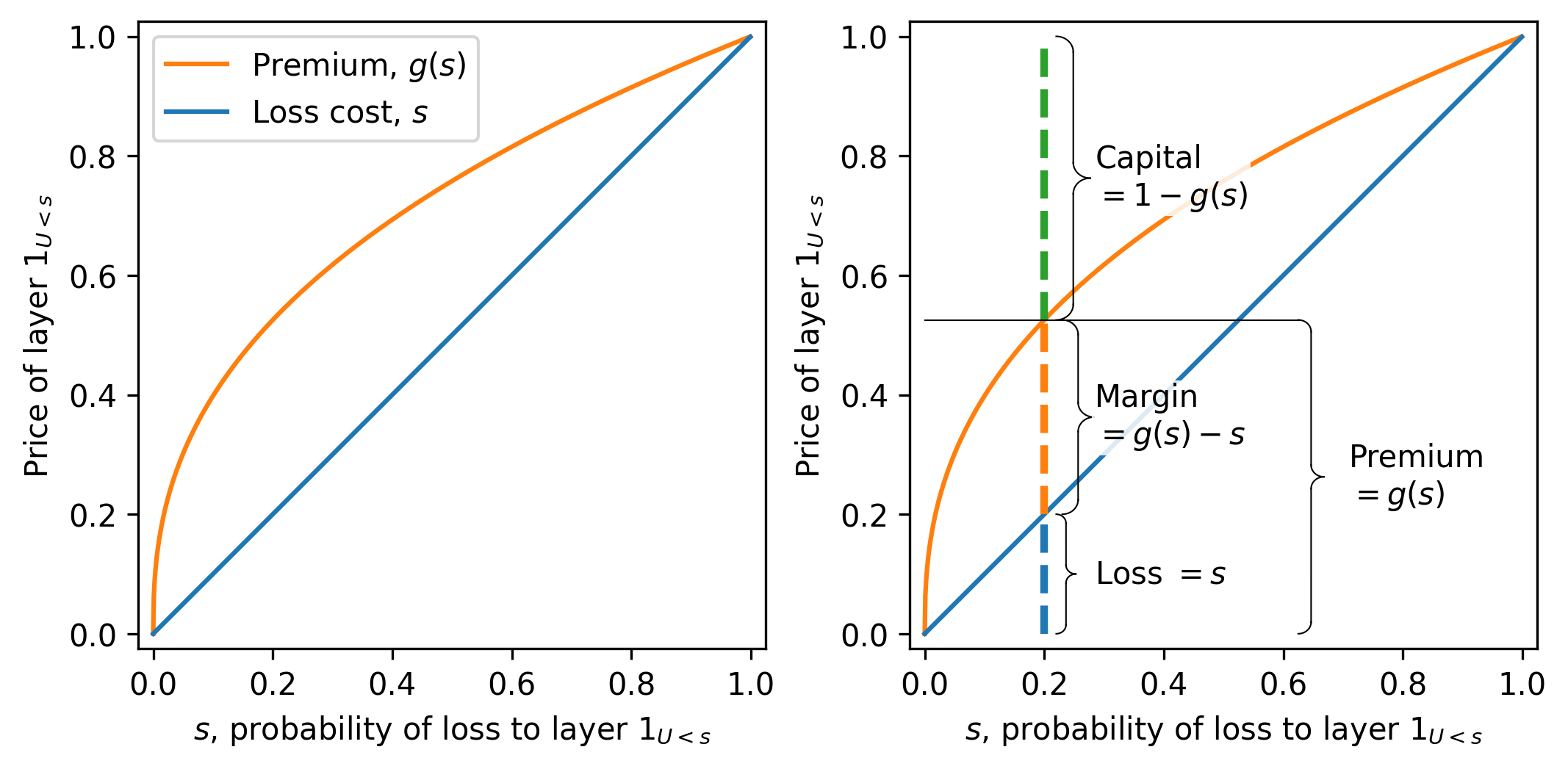
Figure fig-distortion-10-3 illustrates a typical concave distortion. The horizontal axis shows $s$. Various insurance market statistics for the layer can be read off from $g$. The expected loss equals the distance from the horizontal axis to the diagonal, the expected margin from the diagonal to the curve, and the capital from the curve to the top of the figure. The figure height equals 1, the outcome value of the Bernoulli layer in a loss state.

Figure 4.2: A typical concave distortion (left) and insurance interpretation (right). The distortion is a proportional hazard, $g(s)=s^\alpha$ with $\alpha=0.4$. It is quite extreme (bows up considerably from the diagonal), to illustrate the shape clearly.

Condition (1) in the definition does two things. It codifies that certainty is free, and it ensures translation invariance. If we add a certain amount to a risk, its price should go up by exactly that amount. Without Condition (1) translation invariance fails. For example, suppose we used $g(s)=0.1+0.8s$, so that $g(0)=0.1$ and $g(1)=0.9$. Then a sure zero is priced at $0.1$ instead of $0$, and a sure one is priced at $0.9$ instead of $1$. If we try to add one unit of certain payoff to the sure one, we expect the price to move from $0.9$ to $1.9$, but under this $g$ there is no consistent way to represent or price the result. The failure at the endpoints breaks the link between adding certainties and adding their prices, which is why the requirements $g(0)=0$ and $g(1)=1$ are essential.

Condition (2) ensures more likely losses are more expensive.

Condition (3) implies pricing derived from $g$ is subadditive, Definition def-SA. Further, conditions (2) and (3) imply the following important facts about concave distortions (see PIR 10.4 and 10.6 for details.).

$g$ is continuous everywhere except possibly at $s=0$, where there can be a jump up to $g(0+)\ge 0$.
$g$ is differentiable everywhere except for at most countably infinitely many points, where it can have kinks.
$g'(s)\ge 0$ where $g'$ exists, since $g$ is increasing.
The left and right-hand derivatives of $g$ exist everywhere on $(0,1)$, both are decreasing, and the right derivative is less than or equal to the left.
$g$ is twice differentiable almost everywhere, i.e., except for a possibly uncountable set of probability zero.
Since $g$ is concave, $g''(s)\le 0$ where $g''$ exists, in other words, $g$ increases at a decreasing rate.
If $g$ is differentiable then it is concave iff $g'$ is decreasing.

Finally, the interpretation of $g(s)$ as the ask price to write any Bernoulli $s$ means that $g$ can be regarded as a law invariant functional on the set of Bernoulli random variables. sec-040-srms shows how to extend this latter interpretation to positive and general random variables.

4.3.2 Five Representative Distortion Functions

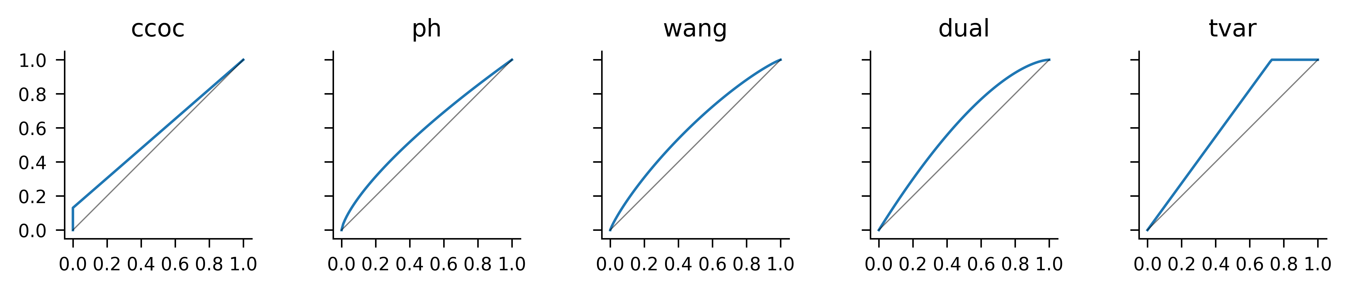
There are many parametric families of concave distortions in the literature, see PIR Ch 11.3 for a sampling. In practice, there are five families worth knowing well.

Constant cost of capital (CCoC), $g(0)=0$ and for $s>0$, g(s) = s+$, where $\nu+\delta=1$, $\nu\ge 0$, and $\delta \ge 0$. It is so named because it prices to a constant cost of capital equal to $\delta/\rho$, Remark rem-040-ccoc. It is more convenient to parameterize in terms of the discount rate $\delta=r/(1+r)$ than the return $r$, because discount ranges from $0$ to $1$ not $0$ to $\infty$.
Proportional hazard (PH), $g(s) = s^\alpha$, $0 < \alpha \le 1$ so named because it act to increase the hazard rate (Dickson et al. 2015).
Wang, $g(s) = \Phi\left(\Phi^{-1}(s)+\lambda\right)$, $\lambda \ge 0$, introduced in Wang (2000). $\Phi$ is the standard Gaussian cumulative distribution function.
Dual, $g(s) = 1-(1-s)^m$, $m\ge 1$.
Tail Value at Risk (TVaR), $g(s) = 1\wedge (s/(1-p))$ for $0 \le p < 1$.

For fixed $s$, the PH increases with decreasing $\alpha$ and the other four increase with their parameter. Figure fig-example-distortions plots examples of each, with broadly comparable parameters. The pictures are consistent with the various properties assumed and asserted above for distortions. Table tbl-the5dists recaps the formulas for each $g$ and shows the parameters used in the plots.

Figure 4.3: Plots of five representative distortion functions. The identity diagonal is shown in blue for reference.

Table 4.1: Formulae and parameters for five representative distortion function families.

Distortion	Formula	Parameter
CCoC	$\nu s+\delta$	$\iota=0.1500$
PH	$s^\alpha$	$\alpha=0.7205$
Wang	$\Phi(\Phi^{-1}(s)+\lambda)$	$\lambda=0.3427$
Dual	$1-(1-s)^m$	$m=1.5951$
TVaR	$1\wedge s/(1-p)$	$p=0.2713$

Remark 4.5. The CCoC distortion prices a Bernoulli $s$ risk to a constant cost of capital $r:=\delta/\rho$ in the following sense. To credibly bear a Bernoulli risk requires assets $a=1$. The insured pays $g(s)$ leaving $Q=1-g(s)=1-(\nu s +\delta)=\delta(1-s)$ funded by capital. The margin equals $M=g(s)-s=\nu s +\delta - s =\delta(1-s)$. Therefore the return on capital is $M/Q = \delta/\nu-r$. $\quad\square$

4.3.3 Concavity and Its Importance

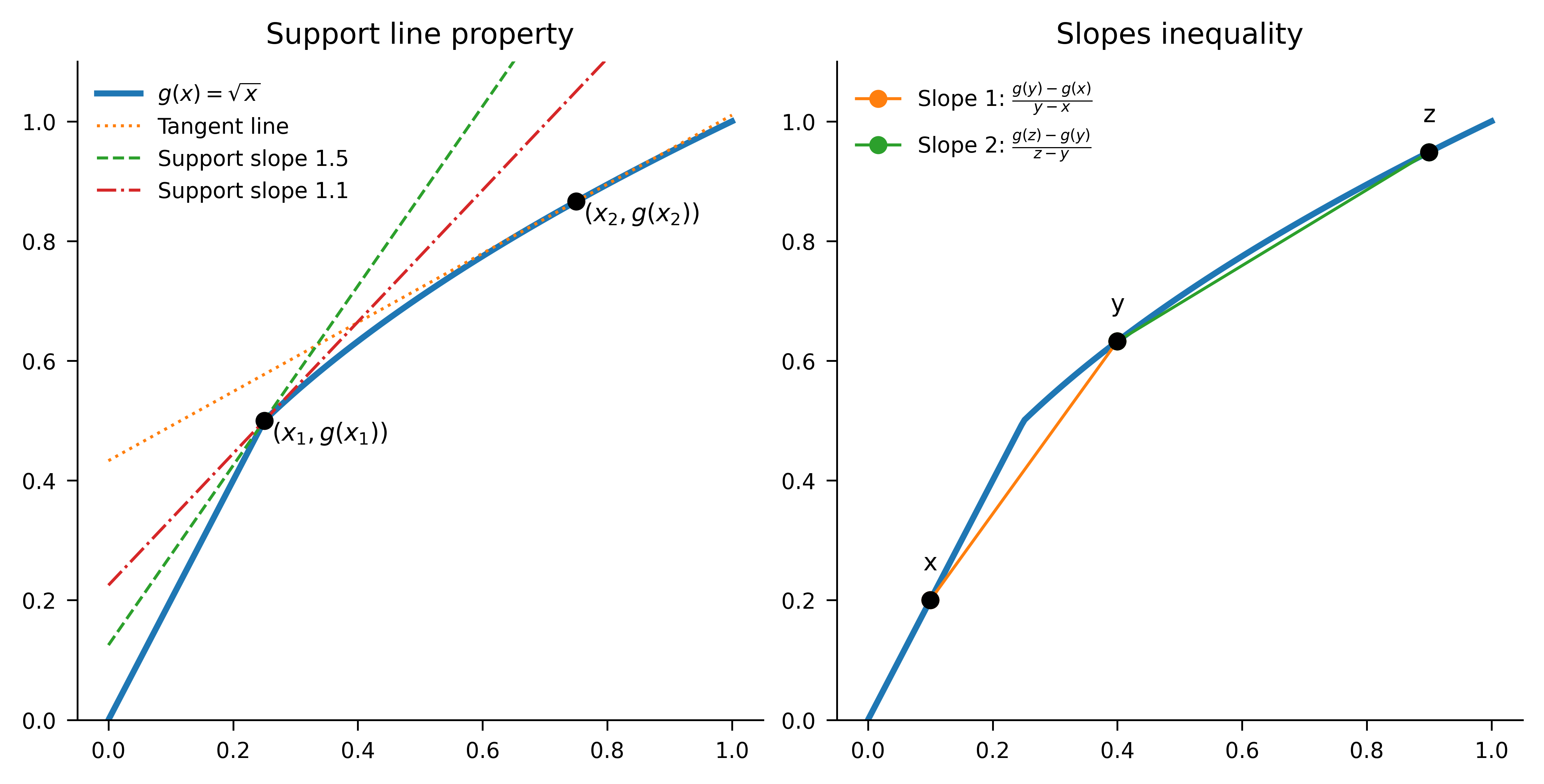
A function $g$ is concave if for all $x,y\in[0,1]$ and all $0<\lambda <1$, \[ \lambda g(x)+(1-\lambda)g(y) \le g(\lambda x+(1-\lambda)y). \] Graphically, this condition means that every chord lies below the graph. Concavity is equivalent to the slopes inequality: for all $0 \le x < y < z \le 1$, \[ \frac{g(y)-g(x)}{y-x} \ge \frac{g(z)-g(y)}{z-y}. \] That is, the secant slopes are non-increasing as you move right. The equivalence can be seen as follows.

Concavity implies the slopes inequality: apply the definition to $y$ as a convex combination of $x$ and $z$; rearrange to get the monotone-decreasing secant slopes.
Slopes inequality implies concavity: fix $x<y<z$ and write $y=\lambda z+(1-\lambda)x$ with $\lambda=(z-y)/(z-x)$. Compare the two secant slopes, substitute $z-y=\lambda (z-x)$ and $y-x=(1-\lambda)(z-x)$, cancel $z-x>0$ to get \[ \frac{g(y)-g(x)}{1-\lambda} \ge \frac{g(z)-g(y)}{\lambda} \] and rearrange.

Concavity has a tangent line interpretation. If $g$ is differentiable at $x$, then for all $y\in [0,1]$, \[ g(y) \le g(x)+g'(x)(y-x), \] i.e., the graph of $g$ lies below its tangent line at every $x$. If $g$ is not differentiable, replace the tangent by any supporting line $L$ at $x$, that is, a line touching the graph of $g$ from above. Then $g$ is concave iff $g$ lies at or below every support line at every point. Figure fig-slopes-chords illustrates these ideas a point where $g$ is differentiable and one where it is not.

Figure 4.4: The slopes and support line definitions of concavity.

To see why the concavity of $g$ is important, consider the function $g(s)=s^2$ which is increasing, has $g(0)=0$ and $g(1)=1$, but is not concave (it is convex). Let’s look at pricing for the two random variables $\{ U < 0.3\}$ and $\{U > 0.7\}$, with $U$ uniform. Both variables have price $g(0.3)=0.09$. Because the two variables are defined with the same $U$, a pool (sum) of the two has the same distribution as $\{ U < 0.6\}$ and by law invariance has price $g(0.6) = 0.36$. Thus, the price of the pool is greater than the sum of the prices of the parts, $2\times 0.09 = 0.18$, contradicting diversification and violating subadditivity. This example shows subadditivity demands \[ g(s+t)\le g(s)+g(t)\qquad(s,t\ge 0,\ s+t\le 1), \] which follows from, but is weaker than, concavity.

Exercise 4.1 Confirm that pricing is subadditive for the PH $\alpha=0.5$ distortion and the same two risks.

Solution 4.1. Each risk has price $g(0.3) = 0.548$ and \[ g(0.6) = 0.775 < 2 \times 0.548 = 1.095. \] $\square$

4.3.4 The Dual of a Distortion

By definition, $g(s)$ is the ask price for a Bernoulli-$s$ loss $X$. We now derive the corresponding bid pricing function using a variation of the argument in Proposition prp-020-bid-ask-relationship. Define $\check g(t)$ to be the bid price for a Bernoulli $t$ loss.

Assume bid and ask prices come from the same internally consistent quoting rule. Suppose an insured buys the Bernoulli $s$ loss $X$ at the ask price $g(s)$, and the insurer hedges (reinsures) by selling the complementary payoff $1-X$. Since $1-X$ is Bernoulli $1-s$, the hedge earns $\check g(1-s)$. Holding $X$ and $1-X$ produces the sure payoff 1, so its price is 1. No-arbitrage therefore implies \[ 1 = g(s) + \check g(1-s). \] Rearranging yields \[ \check g(s) = 1 - g(1-s). \] The bid price function $\check g$ associated with $g$ in this way is called the dual of $g$ (not to be confused with the dual distortion).

Geometrically, the graph of $\check g$ is obtained by a point reflection of the graph of $g$ through $(1/2, 1/2)$; see (REF?). Therefore, $\check g(0)=0$, $\check g(1)=1$, and $\check g$ is increasing. If $g$ is concave, then $\check g$ is convex. Taking the dual twice returns the original function: $\check{\check g} = g$ since $\check{\check g}(s)=1-\check g(1-s)=1-[1-g(1-(1-s))]=g(s)$.

4.3.5 Transformations of $g$ and Their Economic Meaning

A distortion $g:[0,1]\to[0,1]$ is increasing and satisfies $g(0)=0$, $g(1)=1$. There are four symmetries of the unit square that fix the diagonal from $(0,0)$ to $(1,1)$. They act on $g$ as: \[ \begin{aligned} g(s) & \ && \text{(identity)}, \\ \check g(s) &:= 1 - g(1-s) && \text{(dual)}, \\ g^{-1}(t) &:= \inf \{s : g(s)\ge t\} && \text{(generalized inverse)}, \\ \hat g(s) &:= 1 - g^{-1}(1-s) = (\check g)^{-1}(s) && \text{(dual–generalized inverse)}. \end{aligned} \] Table tbl-040-four-transfs shows their action on the point $(s,g(s))$. The inverse and dual transformations swap concavity and convexity; the identity and dual-inverse both preserve concavity and convexity.

Table 4.2: The four symmetries of a square fixing the diagonal and their induced action on distortions.

Square symmetry	Transform	Point action	Induced	Concave/ex
identity	identity	$(s,g(s))$	$g$	preserved
reflect in diagonal $y=x$	inverse	$(g(s),s)$	$g^{-1}$	swapped
rotate $180^\circ$	dual	$(1-s,1-g(s))$	$\check g$	swapped
reflect in anti-diagonal $y=1-x$	dual-inverse	$(1-g(s),1-s)$	$\hat g$	preserved

These four transformations form a commutative group isomorphic to the Klein four-group $V$. Each element is an involution (has order 2). Useful identities include \[ \check{\check g}=g,\quad (g^{-1})^{-1}=g,\quad \hat{\hat g}=g,\quad \check{(g^{-1})}=\hat g. \]

SORT OUT.

The transformations have economic interpretations. We know $g$ represents the ask price and $\check g$ the bid price schedule for Bernoulli risks. The use of the remaining two is presented in REF.

Ask prices include a positive margin and therefore satisfy $g(s)\ge s$. Bid prices include a negative margin and satisfy $\check g(s)\le s$. Moreover, to ensure subadditivity (respectively superadditivity) of the induced pricing functional, $g$ must be concave and $\check g$ convex. The transformation given by rotation of the graph by $180^\circ$, corresponding to $g\leftrightarrow \check g$, preserves the boundary conditions while exchanging concavity and convexity, exactly as required. In particular, any increasing concave (respectively convex) function satisfying $g(0)=0$ and $g(1)=1$ necessarily lies above (respectively below) the diagonal and therefore embeds a positive (respectively negative) margin.

The dual-inverse $\hat g$ admits a natural interpretation when pricing is expressed in the quantile domain. Writing a loss as $X=q(p)$ for $p\in[0,1]$, the distortion pricing functional can be written as an integral over distorted survival probabilities. Geometrically, this corresponds to evaluating the area under the curve $x\mapsto g(S_X(x))$. Rotating this graph by $180^\circ$ induces a new quantile function $\hat q$ satisfying $\hat q(u)=q(p)$ for the unique $p$ such that $1-u=g(1-p)$, that is, $p=\hat g(u)$. Hence \[ \hat q(u)=q(\hat g(u)). \] The dual–inverse therefore acts by reparameterizing the quantile function rather than altering probabilities or outcomes: it combines the buyer–seller reversal (dual) with a change of probability scale (inverse). In this sense, $\hat g$ represents the natural action of bid pricing directly in quantile space.

The dual-inverse transformation reveals a symmetry between the five representative distortions, see REF. It exchanges \[ \text{CCoC} \longleftrightarrow \text{TVaR}, \qquad \text{PH} \longleftrightarrow \text{Dual PH}, \] while the Wang transform is invariant.

Exercise 4.2 Confirm these exchanges.

Solution 4.2. The CCoC and TVaR symmetry is obvious from the picture. For the PH and dual, consider a point $(s, g(s))$ on the graph of PH $g(s)=s^{1/d}$. Its reflected point is \[ (1-g(s), 1-s)= (1 - s^{1/d}, 1-s). \] Under the dual $g(s)=1 - (1-s)^d$ this point maps to \[ \begin{aligned} 1 - s^{1/d} &\mapsto 1 - (1 - [1 - s^{1/d}])^d \\ &\mapsto 1 - (s^{1/d})^d \\ &\mapsto 1 - s \end{aligned} \] as required. To see the Wang is self-reflective, recall that \[ 1-\Phi(z)=1 - \mathsf P(Z \le z) = \mathsf P(Z> z) = \mathsf P(Z\le -z) = \Phi(-z) \] by the symmetries (and continuity) of the normal distribution. Then the point mirrored point $(1-g(s), 1-s)$ maps, under Wang, to \[ \begin{aligned} 1 - \Phi(\Phi^{-1}(s) + \lambda) &\mapsto \Phi[ \Phi^{-1}\{ 1 - \Phi(\Phi^{-1}(s) + \lambda)\} + \lambda ] \\ &\mapsto \Phi[ \Phi^{-1}\{ \Phi(-\Phi^{-1}(s) - \lambda) \} + \lambda ] \\ &\mapsto \Phi[ -\Phi^{-1}(s) - \lambda + \lambda ] \\ &\mapsto \Phi[ -\Phi^{-1}(s) ] \\ &\mapsto 1 - \Phi[ \Phi^{-1}(s) ] \\ &\mapsto 1 - s \end{aligned} \] as required. $\square$

4.3.6 TVaR as Extreme Points and the Kusuoka Correspondence

Before getting to details, here is a potted summary. New terms are defined as they are introduced below. All points in a convex set can be written as weighted sums of extreme points. The set of concave distortion functions and of measures on $[0,1]$ are both convex. TVaR distortions are extreme points (like corners) in former, and Dirac delta measures are extreme points in the latter. (The Dirac delta measure $\delta_x$ put probability $1$ on the single point $x$.) The Kusuoka Correspondence $\Psi$ is a map from the set of measures on $[0,1]$ to the set of concave distortion functions defined by $\Psi(\delta_p)=\mathsf{TVaR}_p$ and then extending by linearity to all measures. Thus, $\Psi$ is a dictionary between a distortion $g$ and a probability measure on $[0,1]$ that gives a representation of $g$ is a weighted sum of TVaRs. The rest of this subsection builds out the details of these ideas.

We start by recalling the standard definitions of convexity and extreme points in a vector space.

Definition 4.3 (Convex Sets and Extreme Points.) Let $V$ be a vector space. A subset $K \subseteq V$ is convex if the line segment connecting any two points in the set lies entirely within the set. That is, for all $x, y \in K$ and $\lambda \in [0,1]$: \[ \lambda x + (1-\lambda)y \in K. \]

An element $e \in K$ is an extreme point if it cannot be decomposed as a non-trivial convex combination of other points in $K$. Formally, $e \in \mathsf{Ext}(K)$ if the equality \[ e = \lambda x + (1-\lambda)y \] with $x, y \in K$ and $\lambda \in (0,1)$ implies that $x = y = e$.

Geometrically, extreme points correspond to the “corners” or “vertices” of the set. For example, in a triangle, the extreme points are the three vertices, and in a disk, the extreme points are its circular boundary. In the triangle, points on the edges are convex combinations of the endpoint vertices, and interior points are combinations of all three vertices. In the disk, points in the interior are combinations of boundary points.

Let $\mathcal{M}$ be the set of Borel probability measures on $[0,1]$, and let $\mathcal{D}_c$ be the set of concave distortion functions $g: [0,1] \to [0,1]$ such that $g(0)=0$, $g(1)=1$, and $g$ is concave. Lebesque measure on $[0,1]$ is denoted $\mathsf P$.

Both $\mathcal{M}$ and $\mathcal{D}_c$ are convex spaces (weighted sums of a distortion is a distortion, weighted sum of probabilities is a probability) and their extreme points correspond.

By Aliprantis and Border (2006) Theorem 15.9, the extreme points of $\mathcal{M}$ are precisely the Dirac measures: \[ \mathsf{Ext}(\mathcal{M}) = \set{ \delta_p : p \in [0,1] }. \]

The extreme points of $\mathcal{D}_c$ are TVaR distortion kernel for $p \in [0,1)$ as: \[ \mathsf{tvar}_p(t) = 1 \wedge \frac{t}{1-p} = \begin{cases} \dfrac{t}{1-p} & 0 \le t < 1-p \\ 1 & 1-p \le t \le 1. \end{cases} \] In the limiting case, $\mathsf{tvar}_1(t)=\set{t>0}$. We can see this using a geometric proof as follows. Consider $\mathsf{tvar}_p$ and $t$ in two regions.

For $t \in [1-p, 1]$ (the flat region), $\mathsf{tvar}_p(t)=1$. If $\mathsf{tvar}_p = \lambda h_1 + (1-\lambda)h_2$ for concave distortions $h_1, h_2$, then $h_1(t)=h_2(t)=1$ on this interval, as 1 is the upper bound of any distortion.
For $t \in [0, 1-p]$ (the linear region), $\mathsf{tvar}_p(t)$ is the chord connecting $(0,0)$ to $(1-p, 1)$. By concavity, any distortion $h$ with $h(1-p)=1$ must satisfy $h(t) \ge \mathsf{tvar}_p(t)$ on this interval.
Since for $\mathsf{tvar}_p$ the weighted average equals the lower bound, we must have $h_1(t) = h_2(t) = \mathsf{tvar}_p(t)$ everywhere.

Thus, $\mathsf{tvar}_p$ cannot be decomposed.

Proposition 4.1 (The Kusuoka Correspondence) There exists a linear bijection $\Psi: \mathcal{M} \to \mathcal{D}_c$ defined by: \[ g(t) = \Psi(\mu)(t) = \int_{[0,1]} \mathsf{tvar}_p(t) \, \mu(dp). \]

Linearity follows from linearity of the integral with respect to the measure.

Lemma 4.1 (Mapping of Extreme Points) Let $\delta_q \in \mathcal{M}$ be the Dirac measure concentrated at $q \in [0,1)$. Then $\Psi(\delta_q) = \mathsf{tvar}_q$.

Proof. By the defining property of the Dirac measure, for any bounded measurable function $f$, $\int f(p) \, \delta_q(dp) = f(q)$. Thus, substituting $\mu = \delta_q$ in the definition of $\Psi$, gives \[ \Psi(\delta_q)(t) = \int \mathsf{tvar}_p(t)\delta_q(dp) = \mathsf{tvar}_q(t) \] the TVaR distortion kernel. $\square$

Since $\Psi$ is linear, it preserves convex structure. Thus we can also deduce that $\mathsf{tvar}$ are extreme from the fact $\delta_p$ are extreme.

4.3.7 The Spectrum of a Distortion

Let $g(t) = \int_{[0,1)} \mathsf{tvar}_p(t) \, \mu(dp)$ be a typical distortion. Differentiating with respect to $t$ yields the spectral function (WHERE DEFINED?): \[ \begin{aligned} g'(t) &= \frac{d}{dt} \int_{[0,1)} 1\wedge \frac{t}{1-p} \, \mu(dp) \\ &= \int_{[0,1)} \frac{1}{1-p} \set{t < 1-p} \, \mu(dp) \\ &= \int_{[0, 1-t)} \frac{1}{1-p} \, \mu(dp). \end{aligned} \]

Remark 4.9. The integral is restricted to $[0,1)$ because the term corresponding to $p=1$ is $\mathsf{tvar}_1(t) = \set{t>0}$. On the open interval $(0,1)$, this function is constant (equal to 1), and thus its derivative is zero. Excluding $p=1$ also avoids the singularity at $\dfrac{1}{1-p}$.

To align this with standard spectral representations, we perform a change of variables. Let $s = 1-p$ represent the significance level (or tail probability). This transformation maps the confidence level $p \in [0, 1-t)$ to the tail region $s \in (t, 1]$.

Let $\nu$ be the image measure of $\mu$ under the map $T(p) = 1-p$. That is, for any Borel set $A$, $\nu(A) = \mu\set{ p : 1-p \in A }$. (If $\mu$ has a density $f$, then $\nu$ has density $h(s)=f(1-s)$; standard change of variables.) Substituting $s$ for $1-p$ in the integral gives \[ g'(t) = \int_{(t,1]} \frac{1}{s} \, \nu(ds). \] If $\mu$ has an atom at $p=1$, $g$ has a jump at $t=0$, and the derivative contains a Dirac delta component. This expression now matches the spectral weight construction in Föllmer and Schied (2016), Prop 4.69. The weight $\phi(t) := g'(1-t)$ at quantile level $t$ accumulates the weights $1/s$ for all components active in the tail (where the significance level $s > t$). We call $\nu$ the TVaR-weight measure. See Simon (2011) Theorem 1.29 for a related result.

The previous derivation constructs $g$ from a known measure. However, in practice, we often start with a desired risk profile $g$ and need to determine its constituent TVaR weights. This inverse problem highlights the second dynamic in our circle of equivalences: the TVaR-weight measure $\nu$ is proportional to the curvature of the distortion.

Since $g'(t)$ is an integral over $(t, 1]$, the Fundamental Theorem of Calculus (generalized to measures) implies that the measure $\nu$ is related to the negative derivative of $g'$ \[ dg'(t) = -\frac{1}{t} \, \nu(dt). \] Rearranging this relates the mixing measure directly to the second distributional derivative of $g$: \[ \nu(dt) = -t \, dg'(t). \tag{4.2}\] Since $g$ is concave, $g'$ is decreasing, so $dg'$ is a negative measure. Thus $\nu$ is a positive measure.

Equation eq-mixing offers a powerful heuristic: highly curved regions of the distortion function correspond to heavy weighting of the TVaR parameters in that region. A pure TVaR is the extreme case: all the “curvature” at one point!

A subtle but important feature of this relationship arises at the endpoint $t=1$. The standard Expected Value principle corresponds to $\mathsf{TVaR}_0$, or $s=1$. Does a given distortion $g$ place any weight on the simple average?

We can detect this by inspecting the terminal slope $g'(1)$. From the spectral integral: \[ \lim_{t \to 1} g'(t) = \nu(\{1\}). \] Because $g$ is concave and $g(t) \ge t$, the slope $g'(1)$ is always between 0 and 1.

If $g'(1) = 0$: The measure places no weight on the mean. The risk measure is entirely driven by tail events (e.g., $\mathsf{TVaR}_{0.99}$).
If $g'(1) > 0$: The measure includes a discrete atom at $s=1$ (the mean) with weight exactly equal to this final slope.

Example 4.1 (The Wang $\alpha=0.5$ Distortion.) Consider the Wang distortion $g(t) = \sqrt{t}$. This function is concave, distorting probabilities to be larger than they are ($g(t) > t$). The terminal slope is $g'(t) = \dfrac{1}{2\sqrt{t}}$, so $g'(1) = 0.5$. This immediately tells us that 50% of the risk measure is simply the expected value ($\mathsf{TVaR}_0$). The curvature is $g''(t) = -\dfrac{1}{4} t^{-3/2}$. Using the curvature formula, the continuous density is $\nu(dt) = -t [-\dfrac{1}{4} t^{-3/2}] dt = \dfrac{1}{4\sqrt{t}} dt$. Integrating this density over $[0,1]$ yields $\int_0^1 \dfrac{1}{4\sqrt{t}} dt = 0.5$. As a result the spectral measure $\nu$ consists of a continuous density $\dfrac{1}{4\sqrt{t}}$ summing to 0.5, plus a Dirac mass of 0.5 at $s=1$. The distortion is an equal mix of the mean and a curvature component.

Example 4.2 (Spectral function and TVaR-weight measures for the five representative distortions.)

Table 4.3: The spectral function and TVaR weighs for the five representative distortions.

Name	$g(t)$	$g'(1-t)$ spectral function	$\mu(dp)$ TVaR weight measure
CCoC	$(\delta + \nu t)\set{t>0}$	$\delta\set{t=1} + \nu\set{t<1}$	$\delta\set{p=1} + \nu\set{p=0}$
PH	$t^a$	$a(1-t)^{a-1}$	$a(1-a)(1-p)^{a-1} \, dt + a\set{p=0}$
Wang	$\Phi(\Phi^{-1}(t) + \lambda)$	$e^{\lambda \Phi^{-1}(t) - \lambda^2/2}$	$-(1-p)g''(1-p) \, dp$
Dual	$1 - (1-t)^b$	$b t^{b-1}$	$b(b-1)(1-p)t^{b-2} \, dp$
TVaR	$1\wedge \dfrac{t}{1-p}$	$\dfrac{1}{1-p} \set{t > p}$	$\delta_{p}$

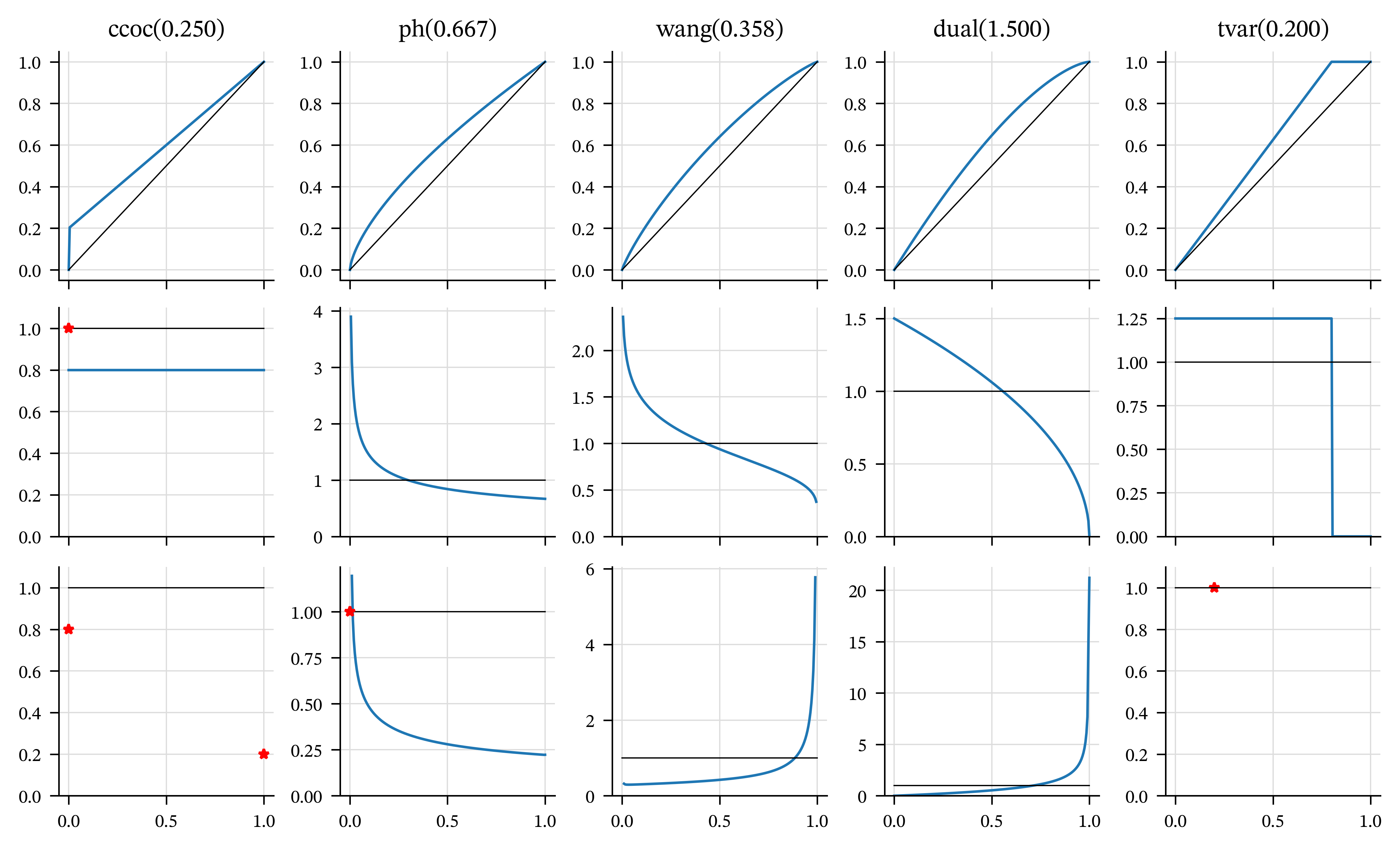
Figure 4.5: The spectral function and TVaR weighs the five representative distortions.

Figure fig-040-wtd-5-rep uses consistent parameter $p$, introduced in Example exm-040-consistent. The first row shows $g$, the second the spectral function $g'(1-t)$, and the third the TVaR-weight measure $-tg''(t)$. In the first two rows small values of $t$ correspond to large losses. In the third row, $t=0$ corresponds to weighting the mean, and $t=1$ to weighting the maximum. Red stars indicate probability masses on particular points. $\quad\square$

See Mildenhall and Major (2022) 10.9 for more examples computing $\mu$ and BLOG-POST for more details.

4.4 Spectral Risk Measures

posts/040-files/040-srms.qmd

This [spectral risk measure] class is very wide and, in our opinion, is sufficient for any practical application of coherent risks. (Cherny and Orlov 2011)

point · point

In this section we show there is a one-to-one correspondence between spectral risk measures (Definition def-020-srm) and concave distortion functions. The correspondence is essentially forced by the axioms. The idea is as follows. If $\rho$ is a SRM, then it is law invariant, comonotonic additive, and coherent, which in turn makes it monotone, translation invariant, positive homogeneous, and subadditive (see definitions in sec-020-risk-measures). Starting from $\rho$ we can use each of these six properties to solve a different piece of the puzzle:

Use law invariance to define a distortion by $g(s)=\rho(A)$ for any set $A$ of measure $s$.
Use comonotonic additivity, positive homogeneity and monotone to extend $g$ to positive random variables using the layer-cake representation.
Use translation invariance to extend to all random variables by writing $X=(k+X) - k$ for $k$ large enough that $k+X$ is positive.
Use subadditivity of $\rho$ to show that $g$ is a concave distortion. This step requires $\Omega$ be atomless.

Conversely, starting with $g$, we:

Define a law invariant functional for positive $X$ by \[ \rho(X)=\int_0^\infty g(\mathsf P(X>x))\,dx \tag{4.3}\] and extending to all $X$ with the $(X+k)-k$ trick.
Use standard properties of integrals to show that $\rho$ is positive homogeneous and translation invariant.
Use the fact that quantiles are linear in comonotonic variables $q_{X+Y}=q_X+q_Y$, and that an increasing function commutes with taking quantiles $f\circ q_X = q_{f\circ X}$ to show that $\rho$ is comonotonic additive.
Use law invariance and the pointwise monotonicity of integrals to show that $\rho$ is monotone.
Use the concavity of $g$ to show $\rho$ is subadditive.

The rest of this section fleshes out these ideas. We present the derivation in detail because it is informative to see how each assumptions is used to drive the conclusions, and because it extends PIR to all random variables, not just positive ones. We start by recalling the survival function expression for the mean and explaining the layer-cake representation.

Exercise 4.3 (Functional notation extends function notation.) This exercise shows that the function and proposed functional notation for $g$ are consistent. Let $X$ be a Bernoulli $s$ random variable. Show that \[ g(s) = \int_0^\infty g(\mathsf P(X>x))\,dx. \]

Solution 4.3. By definition of a Bernoulli risk, \[ \mathsf P(X>x) =\begin{cases} 0 & x<=0 \\ s & 0 < x < 1 \\ 0 & x \ge 1 \end{cases} \] and therefore \[ g(\mathsf P(X>x)) =\begin{cases} 1 & x<=0 \\ g(s) & 0 < x < 1 \\ 0 & x \ge 1. \end{cases} \] The result follows. $\quad\square$

Exercise 4.4 (The CCoC distortion) Show that Equation eq-040-proto-def for a CCoC distortion $g$ applied to bounded, positive $X$ equals \[ g(X) = \nu \mathsf P(X) + \delta \max X. \]

Solution 4.4. Let $m=\max X$ be the upper bound of $X$. Then, using Equation eq-040-ex-ints \[ \begin{aligned} \int_0^\infty g(\mathsf P(X>x))\,dx \int_0^\infty g(\mathsf P(X>x))\,dx &=\int_0^\infty (\nu S(x) + \delta)\set{X\le m}\,dx &=\mathsf P(X) + \delta m. \end{aligned} \] It is important that $g(0)=0$ and that $X$ is bounded in order for the integral to exist. $\quad\square$

4.4.1 The Survival Function Expression for the Mean

Actuaries are familiar with the survival function expression for the mean of a positive integrable random variable \[ \mathsf PX = \int_0^\infty S(x)\,dx \tag{4.4}\] To see why it holds for all integrable $X$ use integration-by-parts, integrating $dF$ to $F$ for $X<0$ and to $-S$ for $X\ge 0$: \[ \begin{aligned} \mathsf PX &= \int_{-\infty}^{\infty} x\,dF_X(x) \\ &= \int_{-\infty}^0 x\,dF_X(x) + \int_0^{\infty} x\,dF_X(x) \\ &= \left(xF(x)\Big\vert_{-\infty}^0 -\int_{-\infty}^0 F_X(x)dx\right) + \left( - xS(x)\Big\vert_0^{\infty} + \int_0^{\infty} S_X(x)\,dx\right) \\ &= -\int_{-\infty}^0 F_X(x)\,dx + \int_0^{\infty} S_X(x)\,dx. \end{aligned} \] The last line relies on $F(-\infty)=S(\infty)=0$.

4.4.2 The Layer-Cake Representation for Positive Random Variables

The layer-cake representation of $X\ge 0$ writes it as the limit of a sum of comonotonic indicator functions. It is an idea introduced to actuaries by Gary Venter.

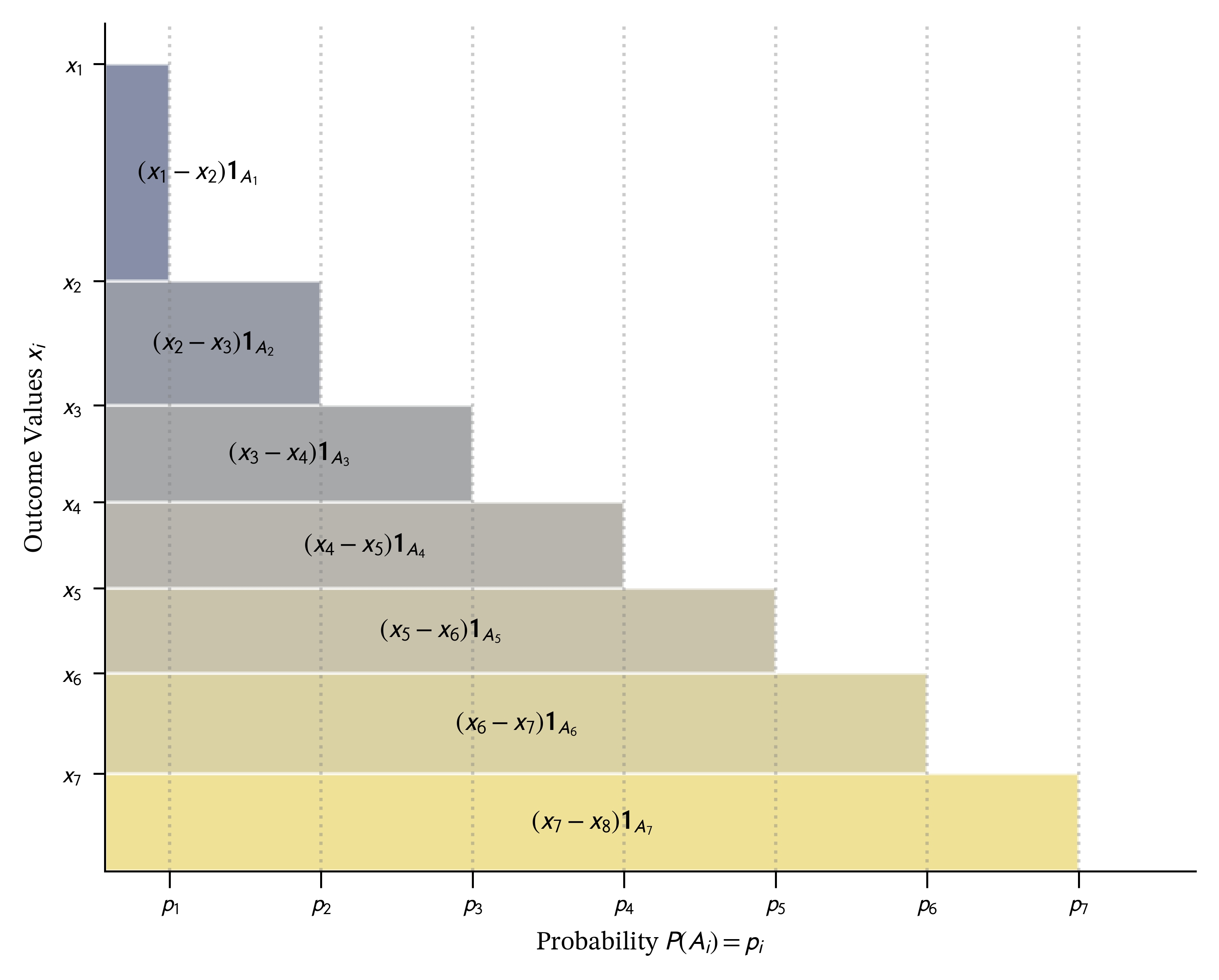
Start with a discrete random variable $X$ taking distinct positive values $x_1 > x_2 > \dots > x_n > 0$. We can explicitly create a sequence of nested sets $A_k := \set{\omega \mid X(\omega) \ge x_k}$, which ensures $A_1 \subset A_2 \subset \dots \subset A_n$. The risk $X$ can then be reconstructed using its “layer-cake” decomposition as a sum of scaled indicator functions on these sets: $X = \sum_{i=1}^n (x_i - x_{i+1}) A_i$, where we define $x_{n+1}=0$, as illustrated in Figure fig-layer-cake. Because the sets $A_i$ are nested, their indicator functions are comonotonic. (Remember, a set is identified with its indicator function.) The diagram looks like a special case, where $X$ is neatly arranged to be decreasing. However, by Ryff’s theorem, we can just re-arrange the sample space to ensure that happens Föllmer and Schied (2016).

Figure 4.6: Decomposition of a discrete random variable into a sum of scaled Bernoulli variables.

We can approximate a general $X \ge 0$ using a sequence of simple functions: \[ X_n = \sum_{k=1}^{N_n} \alpha_{n,k} \mathbf{1}_{\{X > x_{n,k}\}} \tag{4.5}\] where $X_n \uparrow X$ almost surely. By the monotone convergence theorem we can therefore write \[ X = \int_0^\infty \set{X > x}\,dx \] where the integrands are indicator functions \[ \set{X > x}(\omega)=\begin{cases} 1 & X(\omega) > x \\ 0 & \text{otherwise}. \end{cases} \]

4.4.3 Capacities and the Choquet Integral

The relationship between SRMs and distortion functions relies on two new ideas, a capacity and the Choquet integral.

Definition 4.4 A capacity $c$ is a normalized, monotone set function \[ c(\emptyset)=0,\quad c(\Omega)=1,\quad A\subseteq B\Rightarrow c(A)\le c(B). \]

Given a distortion function $g$, \[ A\mapsto g(\mathsf P(A)) \] defines a capacity, which we write $c=g\,\mathsf P$. Not all capacities are of this form, but these are the only ones we consider. Unlike probabilities, capacities are may not be additive.

Definition 4.5 The Choquet integral of a random variable $X$ with respect to a capacity $c$ is \[ \int X\,dc = -\int_{-\infty}^0 [1 - c(\mathsf P(X > x))]\,dx + -\int_{-\infty}^0 c(\mathsf P(X > x))\,dx. \]

The Choquet integral lets the weight of an event depend on an ordering of the sample space by values of $X$. When $c$ comes from a concave $g$

Bad states, the right tail $X\ge 0$, count more than their raw probability because $g(s)\ge s$.
Good states, the left tail $X<0$, count less because $\check g(s)\le s$ (since $\check g$ is convex).

The next proposition confirms that Pollard’s notation works as expected for the TVaR distortion kernels. Define the usual TVaR (or expected shortfall) functional as \[ \mathsf{TVaR}_p(X) := \frac{1}{1-p}\int_p^1 q(s)\,ds \tag{4.6}\] where $q(p) := \inf \{x : S_X(x) \le 1-p\}$ is the lower $p$ quantile function of $X$.

Proposition 4.2 (TVaR Functional.) The functional induced by the extreme TVaR distortion kernel $\mathsf{tvar}_p(s):=1\wedge s/(1-p)$ is the TVaR functional $\mathsf{TVaR}_p$.

Proof. We need to show the functional defined by $\mathsf{tvar}_p(X)$ equals TVaR defined by Equation eq-tvar. This follows using the definition, notational trick, and Fubini’s theorem: \[ \begin{aligned} \mathsf{tvar}_p(X) &= \int_0^\infty \mathsf{tvar}_p(S_X(x))\, dx \\ &= \int_0^\infty 1 \wedge \frac{S_X(x)}{1-p}\, dx \\ &= \int_0^\infty \frac{1}{1-p} \int_p^1 \set{F(x)<t}\,dt\,dx \\ &= \int_0^\infty \frac{1}{1-p} \int_0^1 \set{t \ge p} \set{F(x)<t}\,dt\,dx \\ &= \int_0^1 \frac{\set{t \ge p} }{1-p} \int_0^\infty \set{F(x)<t}\,dx\,dt \\ &= \int_p^1 \frac{1}{1-p} \int_0^\infty \set{F(x)<t}\,dx\,dt \\ &= \frac{1}{1-p} \int_p^1 q(t)\,dt. \end{aligned} \] In detail, as a function of $x$ and $p$, we have: \[ \begin{aligned} \frac{1}{1-p} \int_p^1 \set{F(x)<t}\,dt &= \begin{cases} \dfrac{1 - F(x)}{1-p} & p \le F(x),\ x\ge q(p) \\ 1 & p > F(x),\ x < q(p). \end{cases} \end{aligned} \]

4.4.4 Six Representations of the Choquet Integrals

In this section we give six different integral representations of the Choquet integral.

Theorem 4.1 Let $g \in \mathcal{D}_c$ be continuous distortion with associated measure $\mu$ and spectral derivative $g'$, and define the capacity $c(A):=g(\mathsf P(A))$ and $G_X(x):=1-g(S_X(x))$. Then, the following representations are equivalent: \[ \begin{aligned} g(X) &\stackrel{(a)}{=} \int_{[0,1)} \mathsf{TVaR}_p(X) \, \mu(dp) \\ &\stackrel{(b)}{=} \int_0^1 q_X(t) g'(1-t) \, dt \\ &\stackrel{(c)}{=} \int_0^1 q_X(\hat{g}(s)) \, ds \\ &\stackrel{(d)}{=} \int_0^1 G_X^{-1}(t) \, dt \\ &\stackrel{(e)}{=} \int_0^\infty g(S_X(x)) \, dx \\ &\stackrel{(f)}{=} \int X \, dc \end{aligned} \]

Proof. Throughout, $X\ge 0$ is integrable, $S_X(x)=\mathsf P(X>x)$, and $q_X$ is the (left-continuous) quantile function. Because $g$ is concave and increasing, it is absolutely continuous on compact subintervals of $(0,1)$, has a right-derivative $g'_+$ a.e., and the Lebesgue–Stieltjes measure $dg$ decomposes as $dg = g'_+(u)\,du + dg_s$. To keep notation light, we write $g'(u)$ for $g'_+(u)$ and, when $g$ has a singular part, interpret identities involving $g'(u)\,du$ as the corresponding Stieltjes identities (replace $g'(1-t)\,dt$ by $d(g(1-t))$). Under absolute continuity, the displayed formulas hold literally.

(b) $\iff$ (e): Choquet/survival to spectral. For $x\ge 0$, \[ g(S_X(x))=\int_0^{S_X(x)} g'(u)\,du =\int_0^1 \set{u<S_X(x)}\,g'(u)\,du. \] Insert into (e) and apply Tonelli/Fubini: \[ \int_0^\infty g(S_X(x))\,dx =\int_0^1 g'(u)\int_0^\infty \set{u<S_X(x)}\,dx\,du. \] Now $u<S_X(x)$ is equivalent to $P(X>x)>u$, i.e. $F_X(x)<1-u$. Since $X\ge 0$, \[ \int_0^\infty \set{F_X(x)<s}\,dx = q_X(s),\qquad s\in(0,1), \] because $\{x\ge 0:F_X(x)<s\}=[0,q_X(s))$. With $s=1-u$ this gives \[ \int_0^\infty \set{u<S_X(x)}\,dx = q_X(1-u), \] hence \[ \int_0^\infty g(S_X(x))\,dx =\int_0^1 g'(u)\,q_X(1-u)\,du =\int_0^1 q_X(t)\,g'(1-t)\,dt, \] after the substitution $t=1-u$. This is (b).

(a) $\iff$ (b): mixture to spectral. From the distortion-mixture representation \[ g(t)=\int_{[0,1)} \mathsf{tvar}_p(t)\,\mu(dp), \qquad \mathsf{tvar}_p(t)= 1\wedge \frac{t}{1-p}, \] differentiate under the integral (valid a.e.) to obtain, for a.e. $u\in(0,1)$, \[ g'(u)=\int_{[0,u)} \frac{1}{1-p}\,\mu(dp). \] Substitute into (b) and apply Fubini: \[ \begin{aligned} \int_0^1 q_X(t)\,g'(1-t)\,dt &=\int_0^1 q_X(t)\int_{[0,1-t)}\frac{1}{1-p}\,\mu(dp)\,dt \\ &=\int_{[0,1)}\frac{1}{1-p}\int_0^{1-p} q_X(t)\,dt\mu(dp). \end{aligned} \] Finally, rewrite the inner integral as $\int_p^1 q_X(s)\,ds$ (substitute $s=t+p$), giving \[ \begin{aligned} \int_0^1 q_X(t)\,g'(1-t)\,dt &=\int_{[0,1)} \frac{1}{1-p}\int_p^1 q_X(s)\,ds\mu(dp) \\ &=\int_{[0,1)} \mathsf{TVaR}_p(X)\,\mu(dp), \end{aligned} \] which is (a).

(b) $\iff$ (c): change of variables via the dual–inverse. Let $\check g(t)=1-g(1-t)$ and let $\hat g$ be its upper inverse: \[ \hat g(s)=\sup\set{t\in[0,1]:\check g(t)\le s}. \] Then $\check g(\hat g(s))=s$ for a.e. $s$, and where $\check g$ is differentiable we have \[ \frac{d}{dt}\check g(t)=g'(1-t). \] Using the substitution $s=\check g(t)$ (equivalently $t=\hat g(s)$) yields \[ \int_0^1 q_X(\hat g(s))\,ds =\int_0^1 q_X(t)\,d\check g(t) =\int_0^1 q_X(t)\,g'(1-t)\,dt, \] with the middle expression understood as a Stieltjes integral when $\check g$ is not absolutely continuous. This is (b). Compare Föllmer and Schied (2016) Corollary 4.87.

(d) $\iff$ (e): expectation under the distorted distribution. Let $Y$ have distribution function $G_X$. Then \[ \int_0^1 G_X^{-1}(t)\,dt = \mathsf{P}Y. \] By the tail-sum formula for $Y\ge 0$, \[ \begin{aligned} \mathsf{P}Y &=\int_0^\infty P(Y>x)\,dx \\ &=\int_0^\infty (1-G_X(x))\,dx \\ &=\int_0^\infty g(S_X(x))\,dx, \end{aligned} \] which is (e). Compare Föllmer and Schied (2016) Proposition 4.86.

(f) $\iff$ (e): Choquet notation. For the capacity $c(A)=g(P(A))$, the Choquet integral of $X\ge 0$ is defined by \[ \begin{aligned} \int X\,dc := \int_0^\infty c(\{X>x\})\,dx \\ &=\int_0^\infty g(P(X>x))\,dx \\ &=\int_0^\infty g(S_X(x))\,dx. \end{aligned} \] This is exactly (e), written as (f). $\quad\square$

Remark 4.7. Since $g$ is concave it is differentiable almost everywhere, the points where it isn’t can be ignored in formula (b).

4.4.5 The Spectral Representation Theorem I

In this section we present the first of two representation theorems for spectral measures. This version draws the connection between a SRM and a distortion function. The second is presented in sec-040-srm-ii.

Theorem 4.2 (Spectral Representation Theorem.) Let $\rho$ be defined on the space of bounded random variables on an atomless probability space $\Omega$.

$\rho$ is a loss spectral risk measure if and only if there is a concave distortion function $g$ such that \[ \rho(X) = -\int_{-\infty}^0 \check g(F_X(x))\,dx + \int_0^\infty g(S_X(x))\,dx \tag{4.7}\]
$V$ is a payoff spectral valuation function if and only if there is a unique convex distortion function $\check g$ such that \[ V(Y) = -\int_{-\infty}^0 g(F_Y(x))\,dx + \int_0^\infty \check g(S_Y(y))\,dy \] where $g$ is the dual of $\check g$.

In both cases, the distortion is unique.

Before addressing the proof, it is helpful to interpret equation Equation eq-ru-7-40 for a random variable $X$ that can take both positive and negative values.

We work throughout under the loss sign convention and from the insurer’s perspective. Positive values of $X$ represent payments the insurer must make; negative values represent receipts. To separate these effects, we use the Jordan decomposition, which writes any bounded random variable $X$ as the difference of two non-negative parts: \[ X^+ := \max(X,0), \qquad X^- := \max(-X,0)=-\min(X, 0) \ge 0, \] so that \[ X = X^+ - X^-. \] We regard $X^+$ as a pure loss and $X^-$ as a pure gain. Many insurance contracts are pure losses, while many financing instruments are pure gains, though contracts such as futures or forwards may involve both components depending on how consideration is treated.

Both $X^+$ and $-X^-$ are non-decreasing functions of $X$ and are therefore comonotonic. Since a spectral pricing functional is comonotonic additive, we can price the bundled position by summing the prices of its parts: \[ g(X) = g(X^+) + g(-X^-). \] This expression represents the net ask price of the contract from the insurer’s perspective.

Since $X^+ \ge 0$, its price is the standard Choquet integral, \[ g(X^+) = \int_0^\infty g\bigl(S_X(x)\bigr)\,dx, \] which is the second term in Equation eq-ru-7-40. It corresponds to the loaded cost of the potential payments the insurer must make and carries a positive margin: $g(X^+) \ge \mathsf P(X^+)$.

The term $-X^-$ represents receipts. By bid-ask duality, its ask price satisfies \[ g(-X^-) = -\check g(X^-), \] where $\check g$ is the bid functional dual to $g$. Since $X^- \ge 0$, using Exercise exr-040-f-s-switch shows \[ \check g(X^-) = \int_0^\infty \check g\bigl(S_{X^-}(x)\bigr)\,dx = \int_{-\infty}^0 \check g\bigl(F_X(x)\bigr)\,dx. \tag{4.8}\] Thus the price of the gain component becomes \[ g(-X^-) = -\int_{-\infty}^0 \check g\bigl(F_X(x)\bigr)\,dx, \] which is the first term in Equation eq-ru-7-40. It reflects the discounted credit the insurer gives for potential receipts; equivalently, it embeds a negative margin, since $\check g(X^-) \le \mathsf P(X^-)$.

Putting the pieces together, \[ g(X) = \mathrm{ask}(X^+) - \mathrm{bid}(X^-) = \int_0^\infty g(S_X)\,dx - \int_{-\infty}^0 \check g(F_X)\,dx, \] exactly as in the spectral representation formula.

Economically, this decomposition makes clear how a loss spectral risk measure prices mixed-sign positions. The insurer surcharges what it may have to pay and discounts what it may receive. In practice, most insurance operations involve pure losses sold at a positive margin, while financing activities involve pure gains offered at an attractive (negative-margin) price to investors. These functions are typically handled by separate parts of the firm—underwriting and corporate finance—but equation Equation eq-ru-7-40 shows how they combine coherently within a single pricing functional.

The interpretation for a payoff variable $Y$ under the bid functional $\check g$ is analogous: bid for $Y^+$ minus ask for $Y^-$. In both cases, the same principle applies: surcharge what is paid and discount what is received.

Exercise 4.5 Verify Equation eq-040-f-s-switch.

Solution 4.5. This is a matter of chasing the definitions. $S_{X^-}(x) = \mathsf P(X^- > x)=\mathsf P(-\min(X,0) > x)=\mathsf P(\min(X,0) < -x)=F_{-X^-}(-x)$ and so $\check g(S_{X^-}(x))=\check g(F_{-X^-}(x))$. The result follows by substitution $x\leftarrow -x$ in the first integral in Equation eq-040-f-s-switch. $\quad\square$

Proof. The proof is in several steps. We start by assuming the loss sign convention and work on claim (1).

Part A. From SRM to distortion

Let $\rho$ be a loss SRM.

Step A.1. Identify the distortion. Define $g(s)=\rho(A)$ where $A$ is any set with probability measure $P(A)=s$. This is well-defined due to the law invariance of $\rho$.

Step A.2. Show $g$ is a distortion. SRMs are normalized, so $g(0)=0$ and $g(1)=1$, and monotone, so $g$ is increasing.

Step A.3. Show $g$ is a concave distortion. To show $g$ is concave it is enough to show that $g(y)\ge (g(x)+g(z))/2$ for all $0\le x\le z\le 1$, $y=(x+z)/2$, (Föllmer and Schied 2016, A.1.1). In an atomless space there is enormous flexibility to carve $\Omega$ into disjoint pieces with arbitrary prescribed probabilities, usually with the help of a uniform variable $U$. In particular, set $A=\set{0\le U\le y}$, $B=\set{z-y \le U \le z}$, so that $\mathsf P(A) = \mathsf P(B) = y$, $\mathsf P(A\cap B) = x$ and $\mathsf P(A\cup B) = z$ (draw a picture). The two indicator functions $A\cup B$ and $A\cap B$ are comonotonic, and the sums of indicator functions $A\cup B + A\cap B = A+B$. Therefore, \[ \begin{aligned} g(x) + g(z) &= \rho(A\cup B) + \rho(A\cap B) \\ &= \rho(A\cup B + A\cap B) \\ &= \rho(A + B) \\ &\le \rho(A) + \rho(B) \\ &= 2g(y) \end{aligned} \] by comonotonic additivity and subadditivity. Thus $g$ is concave.

Step A.4. Layer Cake Representation for $X \ge 0$. Applying comonotonic additivity, positive homogeneity, and law invariance to the discrete layer-cake approximation Equation eq-040-discrete-layer-cake gives \[ \begin{aligned} \rho(X) &= \rho\left( \lim_n\sum_i^{N_n} (x_{n,i} - x_{n,i+1})\set{X>x_{n,i}} \right) \\ &= \lim_n \sum_i \rho( (x_{n,i} - x_{n,i+1}) \set{X>x_{n,i}} ) \\ &= \lim_n \sum_i (x_{n,i} - x_{n,i+1}) \rho(\set{X>x_{n,i}}) \\ &= \lim_n \sum_i (x_{n,i} - x_{i+1}) g(s_{n,i}) \end{aligned} \] where $s_{n,i}=\mathsf P(X>x_{n,i})=S_X(x_{n,i})$. We can swap the limit and function because $\rho$ is Lipschitz continuous Lemma lem-020-lipschitz. In the limit, the last line becomes the Riemann sum expression for the integral \[ \rho(X) = \int_0^\infty g(\mathsf P(X>x)) \, dx \tag{4.9}\] showing $\rho(X)$ is the Choquet integral of $X$ with respect to the capacity $g \mathsf P$.

Step A.5. Extension to general $X$. For a general $X$, write $X = (k+X) - k$ where $k=\min X$. Then, apply Step 4 and use translation invariance of $\rho$ and substitution in the integral: \[ \begin{aligned} \rho(X) &= \rho(k+X - k) \\ &= \rho(k+X) - k \\ &= \int_0^\infty g(\mathsf P(k + X > x)) \, dx - k \\ &= \int_0^\infty g(\mathsf P(X > x - k)) \, dx - k \\ &= \int_{-k}^\infty g(\mathsf P(X > x)) \, dx - k \\ &= -\int_{-k}^0 [1 - g(\mathsf P(X > x))] \, dx + \int_0^\infty g(\mathsf P(X > x)) \, dx \\ &= -\int_{-k}^0 \check g(F_X(x)) \, dx + \int_0^\infty g(S_X(x)) \, dx. \end{aligned} \] We can extend the limit on the left hand integral to $-\infty$ because the integrand is zero, giving \[ \rho(X) = -\int_{-\infty}^0\check g(F_X(x)) \, dx + \int_0^\infty g(S_X(x)) \, dx \] as required.

Step A.6. Uniqueness. If $h$ is another distortion satisfying Equation eq-ru-7-40 then by Exercise exr-040-01 is must agree with $g$.

Part B. From distortion to SRM

Conversely, start with a concave distortion function $g$ and define a functional $\rho$ by Equation eq-ru-7-40, the Choquet integral of $X$ with respect to the law invariant capacity $c(A):=g(\mathsf P(A))$.

Step B.1. The Choquet integral is monotone, translation invariant, and positive homogeneous. Monotone follows because if $X\ge Y$ then $\set{Y>x}\subset \set{X>x}$ and $g$ is increasing. Translation invariance follows from the same integral substitution used in step A.5. If $k \ge 0$, then by substitution \[ \int_0^\infty g(\mathsf P(kX>x))\, dx = k\int_0^\infty g(\mathsf P(X>x))\, dx \] and similarly for $X<0$, showing positive homogeneity.

Step B.2. The Choquet integral is comonotonic additive. Let $q_X$ be the quantile function of $X$ and let $f$ be an increasing function. Then $q_{g(X)}=g(q_X)$ (Föllmer and Schied 2016 Appendix A). If $X$ and $Y$ are comonotonic, then $q_{X+Y}=q_X + q_Y$. Comonotonic additivity now follows from Theorem thm-040-six-reps.

Step B.3. If $g$ is concave then $c$ is submodular. Given sets $A$ and $B$, there are three disjoint sets \[ A\cap B,\quad A\setminus B,\quad B\setminus A. \] To prove $c$ is submodular we must show \[ g(A\cup B)+g(A\cap B)\le g(A)+g(B) \] or, re-arranging, that \[ g(A\cup B)- g(B)\le g(A) - g(A\cap B). \tag{4.10}\] The two sides of this inequality are different views of the size of $A\setminus B$. Since $\mathsf P$ is additive, it sees the two as the same size: $\mathsf P(A\setminus B) = \mathsf P(A) - \mathsf P(A\cap B) = \mathsf P(A\cup B) - \mathsf (B)$. Dividing both sides of Equation eq-040-b-2 by this common value reduces us to showing \[ \frac{g(A\cup B)+g(A\cap B)}{\mathsf P(A\cup B) - \mathsf (B)} \le \frac{g(A) - g(A\cap B)}{\mathsf P(A) - \mathsf P(A\cap B)}. \tag{4.11}\] But Equation eq-040-b-3 is exactly the slopes inequality, which holds if and only if $g$ is concave.

Step B.4. If $c$ is submodular then $\rho$ is subadditive. Since $\rho$ is Lipschitz continuous, it is enough to prove this for random variables taking finitely many values. Write $X=\sum_i x_iA_i$ and $Y=\sum_i y_iA_i$ and order the indices so that $x_1+y_1\le \cdots \le x_n+y_n$. Then the $\mathsf Q$ measure from Lemma lem-040-technical has \[ \int X+Y\,dc = \mathsf Q(X+Y) = \mathsf Q(X) +\mathsf Q(Y) \le \int X\,dc +\int Y\,dc. \] This is exactly the impact of diversification: the order of the parts may differ from the order of the sum!

The payoff form follows by applying the loss form to $-V(-X)$. Let $V$ be a payoff SVF. Then $\rho(X)=-V(-X)$ is a loss SRM and so there is a $g$ associated with $\rho$, Equation eq-ru-7-40. For a payoff variable $Y$ be a payoff variable, we have \[ \begin{aligned} V(Y) &= -\rho(-Y) \\ &= -\left( -\int_{-\infty}^0 \check gF_{-Y} +\int_0^\infty gS_{-Y} \right) \\ &= \int_{-\infty}^0 \check g\mathsf P(-Y\le y)\,dy - \int_0^\infty g\mathsf P(-Y>y)\,dy \\ &= \int_{-\infty}^0 \check g\mathsf P(Y\ge -y)\,dy - \int_0^\infty g\mathsf P(Y<-y)\,dy \\ &= \int_{\infty}^0 \check g\mathsf P(Y\ge x)\,(-dx) - \int_0^{-\infty} g\mathsf P(Y<x)\,(-dx) \\ &= - \int_{-\infty}^0 gF_Y + \int_0^{\infty} \check gS_Y, \end{aligned} \] i.e., we swap the roles of $g$ and $\check g$ in Equation eq-ru-7-40.

The proof relies on the following technical lemma, which is a simplification of Föllmer and Schied (2016) Lemma 4.98, tailored to our application where we know the capacity comes from a distortion.

Lemma 4.2 The $A_1,\dots,A_n$ be a partition of $\Omega$ into disjoint measurable sets and let $c$ be a normalized monotone submodular set function associated with the concave distortion $g$. Let $\mathsf Q$ be the measure on the sigma algebra $\mathcal G$ generated by $A_i$ with \[ \mathsf Q(A_k) = c(B_k) - c(B_{k-1}),\qquad B_0:=\emptyset\text{ and } B_k=\bigcup_{j=1}^k A_j,\ k\ge 1. \] Then $\int X\,dc\ge\mathsf Q(X)$ for all $\mathcal G$ measurable $X=\sum_i x_iA_i$, and equality holds if the values of $X$ are arranged in decreasing order $x_1\ge \cdots \ge x_n$.

Proof. First, we show equality for decreasing order. Assume the values of $X$ are ordered such that $x_1 \ge x_2 \ge \dots \ge x_n$. By definition, the Choquet integral is given by: \[ \int X \, dc = \sum_{i=1}^n (x_i - x_{i+1}) c(\{X > x_{i+1}\}) \] (with $x_{n+1}=0$). Since $X$ is sorted, the level sets correspond to the cumulative unions $B_i$: \[ \{X > x_{i+1}\} = A_1 \cup \dots \cup A_i =: B_i. \] Substituting this into the definition and using the telescoping sum yields: \[ \begin{aligned} \int X \, dc &= \sum_{i=1}^n x_i [c(B_i) - c(B_{i-1})] \\ &= \sum_{i=1}^n x_i \mathsf Q(A_i) \\ &= \mathsf Q(X). \end{aligned} \]

Second, we show the inequality for arbitrary orders. Let $Z$ denote the Radon-Nikodym derivative $\dfrac{d\mathsf Q}{d\mathsf P}$. On the partition $A_k$, it is given by the discrete density: \[ Z_k = \frac{\mathsf Q(A_k)}{\mathsf P(A_k)} = \frac{g(\mathsf P(B_k)) - g(\mathsf P(B_{k-1}))}{\mathsf P(B_k) - \mathsf P(B_{k-1})}. \] Geometrically, $Z_k$ represents the slope of the secant line of $g$ over the interval $[\mathsf P(B_{k-1}), \mathsf P(B_k)]$. Since $g$ is concave, it satisfies the slopes inequality, the secant slopes are decreasing: \[ Z_1 \ge Z_2 \ge \dots \ge Z_n. \] Define a random variable $Z$ by $Z(\omega)=Z_k$ if $\omega\in A_k$. Then, \[ \mathsf Q(X) = \mathsf P\left[ X \frac{d\mathsf Q}{d\mathsf P} \right] = \sum_{i=1}^n x_i Z_i \mathsf P(A_i). \] By the Hardy-Littlewood-Pólya rearrangement inequality, this weighted sum is maximized when $X$ and $Z$ are comonotonic (similarly ordered). Since $Z$ is decreasing, the sum is maximized when $X$ is also decreasing ($x_1 \ge \dots \ge x_n$). Thus, the Choquet integral, which corresponds to the expectation under the measure aligned with the decreasing order of $X$, is an upper bound: \[ \int X \, dc \ge \mathsf Q(X). \]

Notation. We write $g(X)$ for functional associated with a distortion function $g$. If $g$ is concave it is a SRM and if convex a SVF.

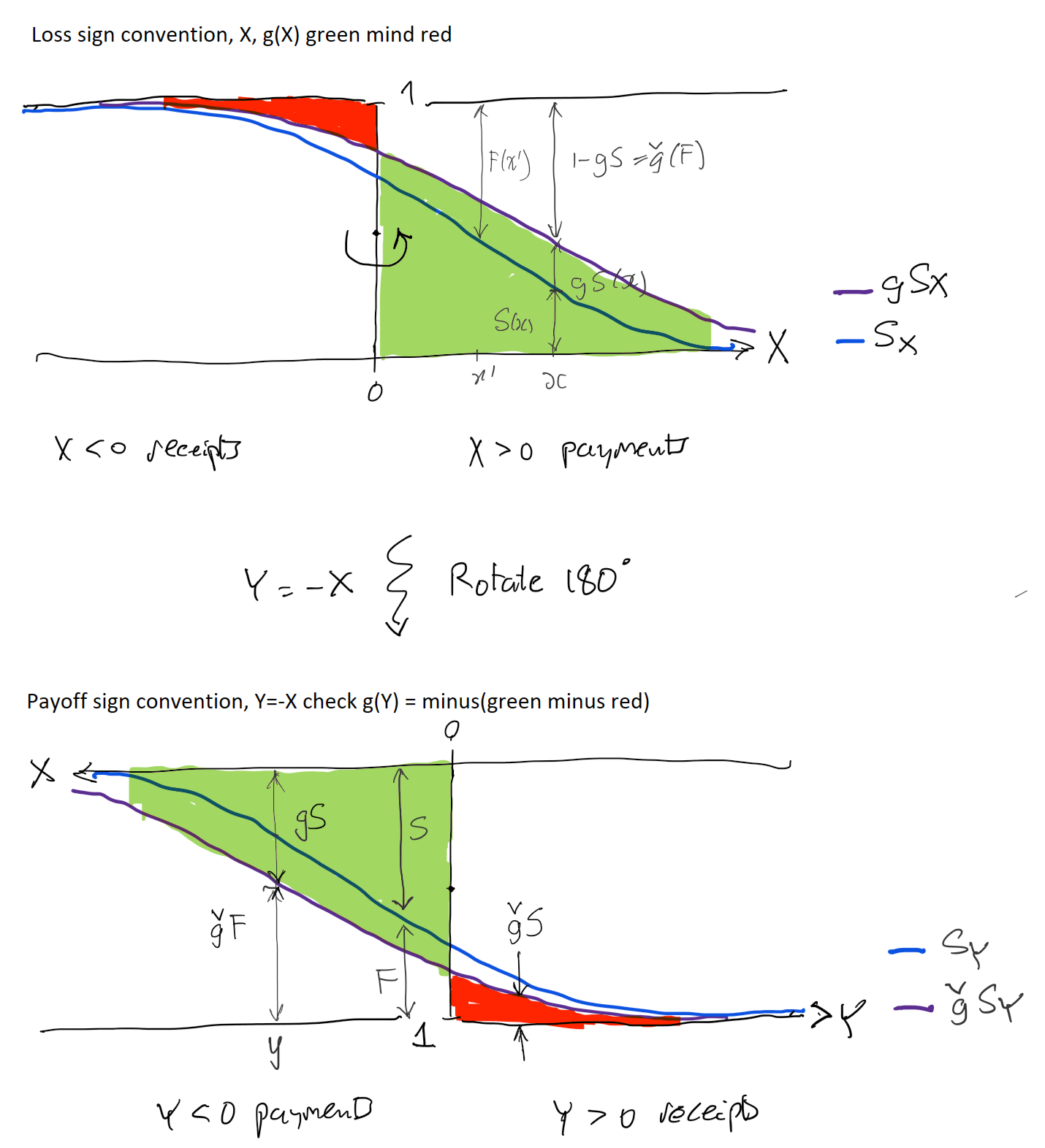
Figure fig-g-general-x illustrates the two calculations, showing that one is transformed into the other by rotating by 180 degrees about the point $(0, 0.5)$, just as a similar rotation about $(0.5, 0.5)$ takes $g$ to $\check g$! It also shows how (top panel) loss payments (positive) have their survival probabilities increased from $s$ to $g(s)>s$, “thickening the tail”, and receipts (negative) have their exceedance probabilities decreased, whereas on the right the opposite holds true. Remember $\check g$ is convex and lies below the diagonal, so $\check g(s)\le s$.

Figure 4.7: Computation of $g(X)$ and $\check g(Y)$, related by a 180 degree rotation of the graph of the survival function.

Remark 4.8 (Historical note). The representation of monotone functionals as integrals with respect to nonadditive set functions originates in Choquet’s capacity theory and the Choquet integral (Choquet 1954) Dellacherie’s monograph on capacities and stochastic processes systematizes the measure-theoretic foundations that later become standard in probability (Dellacherie 1972). Schmeidler then supplies the decisive axiomatic step: comonotonic additivity (plus mild regularity) is exactly what forces a Choquet-integral representation (Schmeidler 1986). In parallel, Yaari’s dual theory reframes the same mathematics as probability distortion rather than utility curvature (Yaari 1987), a viewpoint that enters actuarial pricing via Wang’s distortion premiums and related operators Wang (2000). In mathematical finance, coherence is axiomatized by Artzner, Delbaen, Eber, and Heath in the famous paper Artzner et al. (1999), and Acerbi (2002) identifies the law-invariant, coherent, comonotonic-additive subclass as spectral risk measures (weighted-quantile functionals with an increasing weight profile). Kusuoka’s representation theorem then describes the full law-invariant coherent class (on atomless spaces) as a supremum over a family of AVaR/TVaR-mixtures (equivalently, a supremum over a family of spectra): the comonotonic-additive case corresponds to a single spectrum (hence a unique distortion in your theorem), whereas genuinely non-comonotonic coherent functionals require a nontrivial supremum set (hence, in particular, the “max of at least two SRMs” phenomenon) (Kusuoka 2001). CHECK.

Remark 4.9. The careful reader will notice some possible sloppiness in in the definitions of $F_Y$ and $S_Y$ with regards to less than vs. less than or equal. This results from the definition of value at risk for payoff variables as the negative of the upper quantile, whereas for loss variables it is the lower quantile. CHECK. Marinacci and Montrucchio (2003) shows that the Choquet integral can be define using $g(\mathsf P(X>x))$ or $g(\mathsf P(X>x))$, because the integrands are equal there $g$ is continuous and, as an increasing function, it can have only countably many jumps, which then do not affect the integral.

Example 4.3 This example shows that Theorem thm-040-spectral-rep is not true for a probability space with atoms. It demonstrates that on probability spaces with atoms of unequal probability, law invariance is too weak to enforce the concavity of the distortion function. It constructs a risk measure $\rho$ that is law invariant, comonotonic additive, and coherent, yet that cannot be represented as a mixture of TVaRs. Kusuoka’s representation theorem fails because the atomic structure of the space prevents the construction of a consistent concave distortion.

Consider a simple probability space with two elementary events (atoms) that have unequal probabilities: \[ \Omega = \{\omega_1, \omega_2\}, \quad P(\{\omega_1\}) = 0.1, \quad P(\{\omega_2\}) = 0.9. \] Define the risk measure $\rho$ as the expectation under a different probability measure $Q$, specifically, the uniform measure on these two atoms: \[ \rho(X) = Q(X) = 0.5 X(\omega_1) + 0.5 X(\omega_2). \]

$\rho$ is coherent, because it is linear, which implies subadditivity and positive homogeneity. It is comonotonic additive: linear operators are additive for all variables. And it is law invariant: on $\Omega$ two random variables can only have the same distribution if they map the same values to the same atoms. Thus, $X \sim Y \implies X = Y$ and law invariance holds automatically because no distinct $X$ and $Y$ share a distribution.

If Theorem thm-040-spectral-rep holds, there would be a concave distortion function $g$ such that $\rho(X) = \int X \, d(g P)$. Let’s derive the necessary shape of $g$ using indicator functions (Bernoulli variables). If $X = {\{\omega_1\}}$, a loss of 1 with probability 0.1, then $\rho(X) = 0.5(1) + 0.5(0) = 0.5$ and so $\rho(X) = g(P(\omega_1)) = g(0.1) = 0.5$. Similarly, if $Y = {\{\omega_2\}}$ is a loss of 1 with probability 0.9 then $\rho(Y) = 0.5(0) + 0.5(1) = 0.5 = g(0.9)$. We also know $g(0)=0$ and $g(1)=1$. Thus we have points on the distortion curve \[ (0,0) \to (0.1, 0.5) \to (0.9, 0.5) \to (1,1). \] But, the slope $0 \to 0.1$ equals $(0.5-0)/0.1 = 5$, the slope $0.1 \to 0.9$ equals $(0.5-0.5)/0.8 = 0$ and the slope $0.9 \to 1$ equals $(1-0.5)/0.1 = 5$. This indicates a convex-concave (wobble) shape, showing $g$ cannot be concave. $\quad\square$

Remark 4.10. Each of the six properties of $\rho$ has a essential role in fixing its representation in terms of a distortion function, Table tbl-040-six-rho. Likewise each of the four properties of $g$ is essential and they are combined with properties of integrals, Table tbl-040-six-rep.

Table 4.4: How each of the six properties of a SRM are used to determine its spectral representation.

Property of $\rho$	Why Essential
Law invariant	Allows $g(s)=\rho(A)$
Comonotonic additive	Layer cake representation for sum of indicators
Positive homogeneity	Scaled layer cake
Translation invariant	Extend to negative $(X+k) - k$
Monotone	Continuity for layer cake limit
Subadditivity	Implies $g$ is convex via submodular capacity

Table 4.5: How each of the six properties of a distortion function determine properties of the associated spectral risk measure.

Property of $g$	Why Essential
$g(0)=0$, $g(1)=1$	$c=g\mathsf P$ is normalized.
Increasing	$c$ is monotone
Convex	$c$ submodular and hence $\rho$ is subadditive

Example 4.4 (Subadditive and concave functions.) The subadditivity condition on distortion functions $g(s+t) \le g(s) + g(t)$ is weaker than concavity. For example, the function: \[ g(x) = \begin{cases} 2x & \text{if } x \in [0, 1/4] \\ 1/2 & \text{if } x \in [1/4, 1/2] \\ x & \text{if } x \in [1/2, 1] \end{cases} \] is a subadditive pricing function (check cases based on the intervals for $s$ and $t$). But it is not concave: its slope increases at $s=1/4$. Thus the associated pricing functional should fail to be subadditive. Indeed, apply it to $\{U < 0.5\}$ and $\{ 0.25 < U < 0.75\}$. Each has price $g(0.5) = 0.5$. But the sum has the same distribution as the sum of the comonotonic variables $\{U > 0.25\}$ and $\{U > 0.75\}$, which by comonotonic additivity has value $0.75 + 0.5 = 1.25$. Thus, $g$ is not subadditive as a functional.

Example 4.5 (Spreadsheet Pricing Discrete Choquet Integral.) This example gives a spreadsheet-like computation of $g(X)$ for a discrete random variable taking finitely many positive values $x_i$ with probabilities $p_i$, applying the Choquet integral definition and using Lemma lem-040-technical. The steps are:

Sort by $x_i$ in increasing order. Aggregate ties and sum probabilities.
Compute the survival function at each atom $i$: $S_i=\sum_{j>i} p_j$ (set $S_0=1,\ S_{n}=0$).
Compute the risk-adjusted “probabilities” (they sum to 1): \[ g p_i := g(S_{i-1})-g(S_i)\ \ \ (\ge 0). \]
Mean and price are sum-products: \[ \mathsf P(X)=\sum_i x_i p_i,\qquad g(X)=\sum_i x_i\, g p_i. \]

Table tbl-040-spreadsheet explains a spreadsheet-like implementation of these formulas. See Example exm-040-g-simple-1 and CMM-REF for numerical examples applying this approach.

Table 4.6: Spreadsheet computation of $g(X)$.

Column	Formula
A	$x_i$, sorted in ascending in rows 2 to $n+1$
B	$p_i$, check $p_i\ge 0$ and sum to 1
C	$F_i=\mathrm{SUM}(B2{:}B\set{n+1})$, cumulative probabilities
D	$=1-Ci$, $S_i=1-F_i$, exceedance probabilities
E	$E1=0, Ei = D\set{i-1}$, shifts survival down and prepend 1, $S_0=1, S_{i-1}$
F	$g p_i=g(E_i)-g(D_i)$, difference to obtain risk adjusted probs
G	contribution $=A_i\times F_i$
G total	$g[X]=\mathrm{SUM}(G)$.

Example 4.6 (Pricing Uniform Random Variables.) Let $U$ be a standard uniform $U$ on $[0,1]$ with $S_U(p)=1-p$. This example computes $g(U)$ across the five representative $g$.

The TVaR price equals $(1 + p)/2$ by definition or integrating $g(s)=s / (1-p)\wedge 1$ between $0$ and $1$ to get $(1-p)/2 + p=(1+p)/2$ if you prefer.
The CCoC price is $(1-\delta)\mathsf PU + \delta\max U = (1-\delta)/2 + \delta = (1 + \delta)/2$.
For the dual $g(s)=1-(1-s)^b$ and \[ g(U) = \int_0^1 g(S(s))\,ds = \int_0^1 1-s^b\,ds = b/(b+1). \]
For the PH $g(s)=s^a$ and the integral equals $1/(1+a)$,
The Wang case, $g(s)=\Phi(\Phi^{-1}(s)+\lambda)$ is a little more involved. Let $Z$ and $N$ be independent standard normal variables, then \[ \begin{aligned} g(U) &= \int_0^1 \Phi(\Phi^{-1}(s) + \lambda)\,ds \\ &= \int_{-\infty}^\infty \Phi(z+\lambda)\phi(z)\,dz \\ &= \mathsf E[\Phi(Z+\lambda)] \\ &= \int_{-\infty}^\infty \mathsf P(N \le z+\lambda)\phi(z)\,dz \\ &= \int_{-\infty}^\infty \mathsf P(N \le Z+\lambda \mid Z=z)\phi(z )\,dz \\ &= \mathsf P(N \le Z+\lambda) \\ &= \mathsf P(N - Z \le \lambda) \\ &= \Phi(\lambda / \sqrt 2) \end{aligned} \] because $N-Z$ is normal with mean zero and variance $2$.

Example 4.7 (Consistent Distortion Parameterizations.) The parameterizations given in sec-040-five-reps are awkward to work with and hard to compare because they have different ranges and are not all monotone with risk aversion. To address these shortcomings, we can use an more consistent parameterization defined by equalizing pricing for a reference random variable. We use the uniform as a reference because it is bounded, which allows full capitalization, and the relevant integrals are easy to compute, see Example exm-040-uniform.

For each of the five representative distortions Table tbl-equiv-usual shows the standard parameter name from sec-040-five-reps, and an expression for that parameter in terms of the common $p$ determined by equating the price expression in the last column with that for the TVaR. For CCoC, $\delta=p$. For the dual, equating $(1+p)/2$ with $b/(1+b)$ gives $b=(1+p)/(1-p)$. It can be helpful to think of the dual in terms of a parameter $b:=1/a$ with range $[0,1]$ and mean $1/(1+a)$. Similarly, for the PH $a=(1-p)/(1+p)$, showing that $a$ is the reciprocal of the dual parameter $b$. Finally for the Wang \[ \dfrac{1+p}{2} = \Phi(\lambda / \sqrt 2) \implies \sqrt2\Phi^{-1}\left(\dfrac{1+p}2\right). \]

Table 4.7: Parameters for the five representative distortions yielding the same price for a standard uniform variable.

Distortion	Parameter	Parameter in $p$	Price

TVaR	$p$	$p$	$\dfrac{1+p}{2}$
Dual	$b$	$\dfrac{1+p}{1-p}$	$\dfrac{b}{1+b}$
Wang	$\lambda$	$\sqrt2\Phi^{-1}\left(\dfrac{1+p}2\right)$	$\Phi\left(\dfrac\lambda{\sqrt2}\right)$
PH	$a$	$\dfrac{1-p}{1+p}$	$\dfrac1{1+a}$
CCoC	$\delta$	$p$	$\dfrac{1+\delta}2$

Table tbl-equiv-usual gives a way to create examples of distortions that are balanced in that each has the same price for the uniform distribution. These are useful in constructing examples. Simply select $p$ in $[0, 1]$ and use the five distortions with parameters given by the second column (in terms of $p$) in Table tbl-equiv-usual.

The ordering TVaR to CCoC corresponds most tail-centric (TVaR is cheapest for tail risk, CCoC most expensive) to tail-phobic (TVaR is most expensive for body risk, CCoC cheapest). In all cases higher $p$ corresponds to a higher price, $p=0$ to the mean and $p=1$ to the maximum.

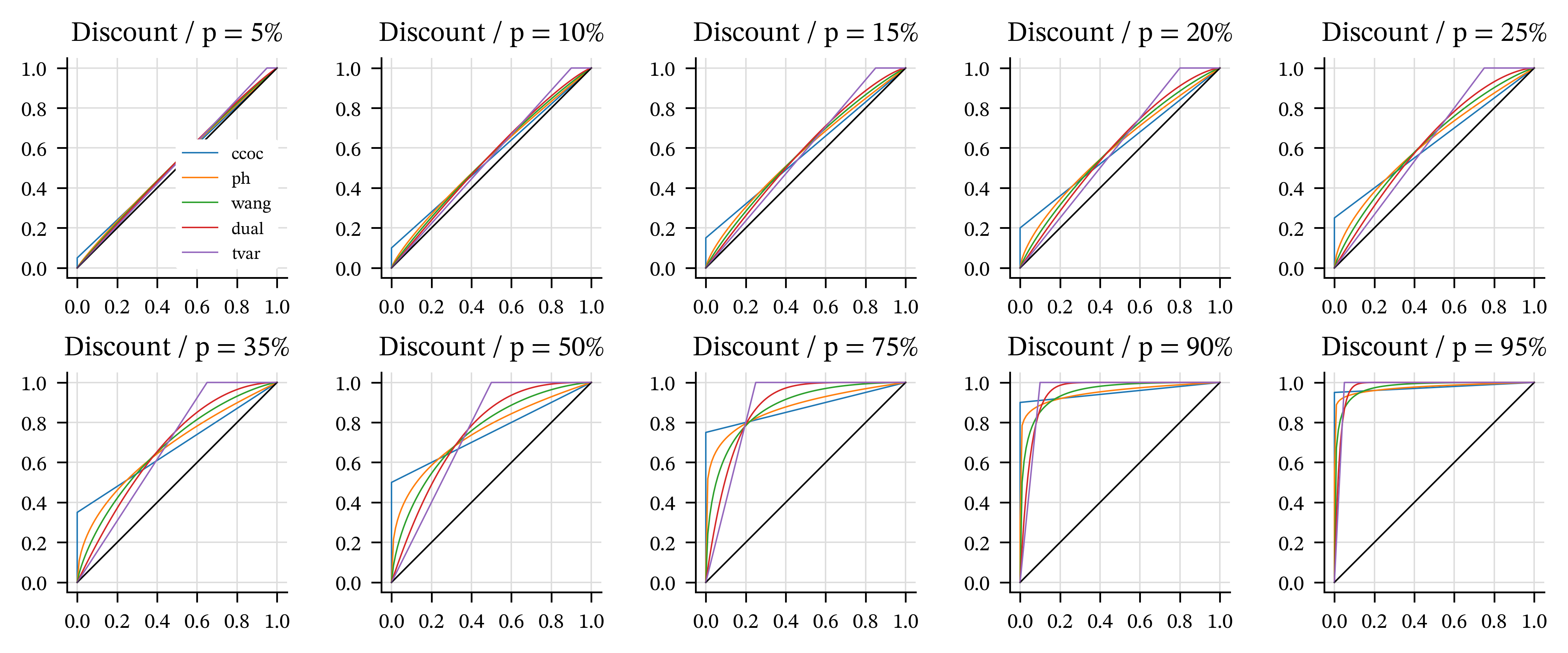
Table tbl-param shows the parameters for a range of $p$ values. Remember, $p$ corresponds to the TVaR $p$ and to the discount rate for CCoC. Thus, a reasonable pricing range is less than about 25% and a reasonable capital measure range is above 90%. Figure fig-param shows the corresponding distortion functions. These parameter ranges and correspondences are a handy reference for deciding reasonable test distortions. The graphs illustrate the symmetries discussed in sec-040-transformations. $\quad\square$

Table 4.8: Parameters of distortions pricing a uniform the same as TVaR $p$ or CCoC with discount $p$, for a range of $p$ values. Column $r$ shows the corresponding CCoC return $r=p/(1-p)$.

p	r	ccoc	ph	wang	dual	tvar
5.0%	5.3%	0.05	0.905	0.0887	1.11	0.05
10.0%	11.1%	0.1	0.818	0.178	1.22	0.1
15.0%	17.6%	0.15	0.739	0.267	1.35	0.15
20.0%	25.0%	0.2	0.667	0.358	1.5	0.2
25.0%	33.3%	0.25	0.6	0.451	1.67	0.25
35.0%	53.8%	0.35	0.481	0.642	2.08	0.35
50.0%	100.0%	0.5	0.333	0.954	3	0.5
75.0%	300.0%	0.75	0.143	1.63	7	0.75
90.0%	900.0%	0.9	0.0526	2.33	19	0.9
95.0%	1900.0%	0.95	0.0256	2.77	39	0.95

Figure 4.8: Plots of distortions pricing a uniform the same as TVaR $p$ or CCoC with discount $p$, for a range of $p$ values.

4.4.6 Calibrating Distortions to Market Pricing

It is easy to calibrate a single-parameter family of distortions to achieve a target price on a given risk. Simply use the Newton-Raphson method, or bisection method. The five representative distortions all price monotonically with parameter making numerical methods very reliable. The aggregate.Portfolio class has a built in method to calibrate using this method. The price can be expressed as a target loss ratio or return on equity, and equity levels can be specified directly or by giving a return period probability. See REF-HELP.

4.4.7 The Spectral Representation Theorem II

In this section we present the second of two representation theorems for spectral measures; the first, in sec-040-srm-i, draws the connection between a SRM and a distortion function. This one applies more general results from the theory of coherent risk measures to SRMs specifically. It is needed in the next section to calculate and interpret the natural allocation. Throughout, $X$ denotes a loss (larger is worse) and $(\Omega,\mathcal F, \mathsf P)$ is an atomless probability space.

There are three equivalent ways to view a spectral risk measure (SRM):

a primal form, as a weighted average of quantiles (the spectrum budget view),
a dual form, as a worst-case expected value over a set of probability measures $\mathcal Q$ (the scenario or stressed measure view), and
a risk adjusted probability form, using the contact (subgradient) function $Z = d\mathsf Q/d\mathsf P$ to effect the adjustment.

In 3., $Z$ is chosen to attain the dual bound, and it acts like a tangent.

By REF (b) we know that for positive $X$, a distortion defines an SRM via \[ g(X) = \int_0^1 q_X(u)\,d\check g(u), \] interpreted as a Stieltjes integral.

When $g$ is absolutely continuous, write $d\check g(u)=\phi(u)\,du$ with $\phi(u)=g'(1-u)$ a.e. Then \[ g(X) = \int_0^1 q_X(u)\,\phi(u)\,du, \] and $\phi$ is a spectrum: $\phi\ge 0$, $\int_0^1\phi(u)\,du=1$, and $\phi$ is nonincreasing.

The dual representation writes the operator $g$ as a supremum of expectations under alternative measures.

Theorem 4.3 (Dual representation with explicit densities.) Let $g$ concave distortion and let $g(X)$ denote the associated SRM. Then there exists a set of probability measures $\mathcal Q$ such that \[ g(X) = \sup_{\mathsf Q\in\mathcal Q} \mathsf Q(X) = \sup_{Z\in\mathcal Z} \mathsf P(XZ), \tag{4.12}\] where $\mathcal Z$ is the set of Radon–Nikodym derivatives $Z=d\mathsf Q/d\mathsf P$ that satisfy:

$Z\ge 0$ and $\mathsf P(Z)=1$ (so $\mathsf Q$ is a probability), and
the spectral budget (majorization) constraint \[ \int_t^1 q_Z(s)\,ds \le g(1-t),\qquad \text{for all } t\in[0,1]. \]

Theorem thm-040-dual-rep says the dual feasible $Z$ are exactly those functions whose integrated quantiles sit below the distortion curve. That is, you are allowed to “tilt” probability toward adverse scenarios (large $X$), but only up to the distortion budget $g$. The more concave $g$ is (the more risk averse), the larger the allowed tail mass of $Z$.

The dual representation is most useful when you identify the optimizers $\mathsf Q^\star$ (or $Z^\star$). These are the contact objects: they define the tangent supporting hyperplane to the operator $g$ at $X$.

Definition 4.6 (Subdifferential and contact function.) For a SRM $g$, the subdifferential at $X$ is \[ \partial g(X):=\set{Z\in L^1 \mid g(Y)\ge g(X)+\mathsf P(Z(Y-X)) \ \text{for all }Y}. \] A density $Z^\star\in\mathcal Z$ is a contact function for $X$ if it attains the supremum: \[ g(X)=\mathsf P(XZ^\star). \]

Any $Z\in\partial g(X)$ can be thought of as defining a tangent line to $g$ at $X$. All contact functions are subgradients; conversely, if the supremum in Equation eq-040-dual-rep-def is attained then subgradients correspond to maximizers (Delbaen 2000 Theorem 17). In turn, the max/sup condition holds provided $g$ is continuous at $0$.

For SRMs, the optimizer contact function $Z^\star$ has three linked properties. First, it is a function of $X$, or $X$-measurable. Moreover, its dependence on $X$ takes a particular form, expressed via the second property: it is comonotonic with $X$ and has the worst-case coupling. Among all feasible $Z$, the one maximizing $\mathsf P(XZ)$ can be taken comonotonic with $X$. Concretely, on an atomless space you can represent $X=q_X(U)$ for a uniform $U$, and then the worst-case $Z$ has the form \[ Z^\star = q_{Z^\star}(U), \] so large losses align with large densities. This is the Hardy–Littlewood rearrangement principle. If it did not hold, you could re-arrange the integral (a sum-product) to obtain a larger total, which contradicts the definition of $Z^\star$ as a contact function.

Third, the constraint \[ \int_t^1 q_{Z^\star}(s)\,ds \le g(1-t) \] binds where it matters most. Informally, $Z^\star$ spends as much of the distortion budget as possible on the upper tail positions that carry the largest values of $q_X(\cdot)$. Where $g$ has “kinks” (changes in slope), those become natural places where the optimal $q_{Z^\star}$ changes regime—this is the quantile-space analogue of tangency conditions in finite-dimensional convex optimization.

In short: $Z^\star$ is a subgradient because it both aligns with $X$ and makes best use of the tail amplification allowed by $g$.

The final lemma of this section presents an important characterization of contact functions as sub-differentials.

Proposition 4.3 Let $g$ be a SRM with set of test densities $\mathcal Z$. Then $Z \in\partial g(X_0)$ if and only if $Z\in\mathcal Z$ and $g(X_0) = \mathsf P(X_0Z)$ is a contact function

Proof. Suppose $Z\in\mathcal Z$ and $g(X_0)=\mathsf P(X_0Z)$. Then for all $Y$ \[ \begin{aligned} g(X_0+Y) &=\sup_{Z'\in\mathcal Z} \mathsf P((X_0+Y)Z') \\ &\ge \mathsf P((X_0+Y)Z) \\ & = \mathsf P(X_0Z) + \mathsf P(YZ) \\ &= g(X_0) + \mathsf P(YZ) \end{aligned} \] and so $Z\in partial g(X_0)$. This is the easy direction: contact functions are subgradients.

Conversely, let $Z\in \parital g(X_0)$. First we claim $Z$ is a probability density, i.e., $Z\ge 0$ and $\mathsf PZ=1$. This can be seen as follows. If $Y\le 0$ then $X\ge X+Y$ and so $g(X)\ge g(X+Y)\ge g(X)+\mathsf P(YZ)$. Note that unlike subadditivity, the subdifferential gives a helpful inequality $g(X+Y)\ge$ something. Hence $\mathsf P(YZ)\le 0$, i.e., $\mathsf P((-Y)Z)\ge 0$ for $-Y\ge 0$ and so $Z\ge 0$. Now take $Y=c\in \mathbb R$. By translation invariance, $g(X) + c = g(X+c)\ge g(X) + \mathsf P(cZ)$, and so $c\ge \mathsf P(cZ)$. If $c\ge 0$ this implies that $\mathsf P(Z)\le 1$ and if $c \le 0$ that $\mathsf P(Z)\ge 1$. Hence $\mathsf P(Z)=1$. We conclude $Z$ is a probability density.

Next we show $Z\in\mathcal Z$ and $g(X_0)=\mathsf P(X_0Z)$. Let $\lambda\in\mathbb R^+$. Then by definition of the subdifferential and for any $Y$, using positive homogeneity, \[ \begin{aligned} g(X_0+\lambda Y) &\ge g(X_0) + \lambda \mathsf P(YZ) \\ \implies g(X_0/\lambda + Y) &\ge g(X_0)/\lambda + \mathsf P(YZ) \\ \implies g( Y) &\ge \mathsf P(YZ) \end{aligned} \] as $\lambda\to\infty$ and so $Z\in\mathcal Z$. Here we use the fact $g$ is continuous with respect to the uniform topology. Finally let $Y=-X_0$, \[ \begin{aligned} 0 = g(0) &= g(X_0 - X_0)\\ &\ge g(X_0) -\mathsf P(X_0Z) \\ \implies \mathsf P(X_0Z) &\ge g(X_0) \end{aligned} \] and so $g(X_0) = \mathsf P(X_0Z)$.

4.5 The Natural Allocation

posts/040-files/060-na.qmd

point · point

In this section, we present the natural allocation of a spectral risk measure, so-called because it entails no additional choices, is consistent with financial, economic, and game theories, and is additive. Moreover, under fairly general assumptions, it equals the marginal cost allocation, an important property making it easy to interpret and use. The natural allocation follows the finance philosophy adjust the probabilities and then act risk neutral. The natural allocation is discussed in Delbaen (2000), Tsanakas and Desli (2003), Föllmer and Schied (2016), though not under that name.

The presentation is a simplified version of PIR chapter 14. We focus on discrete $X$ and work our way around the possibility of default rather than confronting it head-on. According to broker reports, there is over USD100 billion alternative capital in the reinsurance market. That capital supports high margin business that is usually written on fully collateralized, default-free basis. Therefore we can conclude that margin does not rely on default in any way! Throughout, $g$ is a concave distortion, and we use the same notation for the associated spectral risk measure, $X$ is a bounded random variable, and we use the loss sign convention unless noted otherwise.

4.5.1 Preliminary Definition of the NA

Theorem thm-040-six-reps version (b) shows that $g(X)$ can be computed as a re-weighted expected value, where probabilities are adjusted by a factor $g'(S(x))$. Lemma lem-040-technical gives an algorithm for discrete (simulation) $X$, again involving an adjusted probability. The adjusted probability is denoted $\mathsf Q$, following finance conventions. The ratio of adjusted to objective probabilities is a random variable denoted $Z$ and is called a contact function (Definition def-040-subdiff) or the Radon Nikodym derivative. In the discrete case, the probability adjustment factor is given by an approximation to the slope of $g$. Thus, in general, we can write: \[ Z = Z(X) = \frac{d\mathsf Q}{d\mathsf P} = \begin{cases} g'(S(X)) & \text{if $X$ is continuous} \\ \dfrac{g\,\mathsf P(B_i)-g\,\mathsf P(B_{i-1})}{\mathsf P(B_i) - \mathsf P(B_{i-1})} & \text{if $X$ is discrete} \end{cases} \tag{4.13}\] using notation from Lemma lem-040-technical. With $Z$ in hand, \[ g(X) = \mathsf P(XZ) = \mathsf P\left(X \frac{d\mathsf Q}{d\mathsf P}\right) \tag{4.14}\] as a risk adjusted expected value.

Contact function random variables are very important in the analysis. Three important properties follow from their definition: Here is the formal definition.

$Z\ge 0$
$\mathsf P(Z) = 1$
$g(X) = \mathsf P(XZ)$

The contact function $Z$ tells us how much we care about losses from each scenario. The form of $Z$ from Lemma lem-040-technical explains the process most clearly. The outcome values determine an ordering of the sample space. Because $c=g\,\mathsf P$ is submodular and not additive, this order matters. The marginal impact $g\,\mathsf P(B_i)-g\,\mathsf P(B_{i-1})$ decreases as the size of $B_{i-1}$ increases. Each $X$ gets its own adjustment $Z$, where we care most about the largest loss, then the next largest, and so forth.

Delbaen observed that the expectation Equation eq-g-exz makes it “very natural” to allocate an amount \[ a_i = \mathsf{P}(X_i Z) = \mathsf{Q}(X_i) \] part of $g(X)$ to unit $i$ (Delbaen 2000, 33). Thus motivated, we call this the natural allocation of $g$ at $X$ to $X_i$ and denote it $g_X(X_i)$. It is an additive allocation because expectation is linear \[ g(X) = \mathsf{Q}(X) =\mathsf{Q}\sum_i X_i= \sum_i \mathsf{Q}(X_i) = \sum_i a_i. \] The natural allocation process can be applied to any coherent or sublinear risk measure [PIR Ch 14], but it is particularly simple for SRMs where it is easy to write down $Z$ explicitly.

More generally, if $X$ has a mixed distribution with mass points at $\{y_j\}$ and $g$ is continuous then there are jumps $S(y_j-)-S(y_j) =\mathsf P(X=y_j)$ at a finite or countably infinite number of points. Integration by parts also applies to Riemann-Stieltjes integrals with jumps, Hewitt (1960): \[ \begin{aligned} g(X) &= \int_0^\infty g(S(x))\,dx \nonumber \\ &= \int_0^\infty xg'(S(x))f(x)dx \nonumber \\ &\qquad +\ \sum_j y_j\frac{g(S(y_j-))-g(S(y_j))}{S(y_j-)-S(y_j)}\,\mathsf P(X=y_j) \nonumber \end{aligned} \] where we see a new summation term representing that part of the expectation contributed by the distorted jumps. We have written out the denominator $S(y_j-)-S(y_j)$ and the canceling factor $\mathsf P(X=y_j)$ explicitly in order to represent the ratio as $Z(y_j)$. In this case, \[ Z(x)=\begin{cases} g'(S(x)) & S\text{\ is continuous at\ } x \\ \dfrac{g(S(x-))-g(S(x))}{S(x-)-S(x)} & S\text{\ has a jump at\ } x \end{cases} \tag{4.15}\] making the connection between the two parts of Equation eq-z-def clearer.

Example 4.8 (CoTVaR.) The idea behind so-called co-measures such as coTVaR is the same as the natural allocation. Assume $\mathsf P(X=\mathsf{VaR}_p(X))=0$ for simplicity so that \[ \mathsf{TVaR}_p(X) = \mathsf P(X \mid X > \mathsf{VaR}_p(X) ). \] The TVaR contact function $Z=\dfrac{d\mathsf{tvar}_p}{ds}(1-s)$ multiplies the probability of an outcome $x$ by $1/(1-p)$ if $x>\mathsf{VaR}_p(X)$ and sets the probability of other outcomes equal to zero. The corresponding risk adjusted probability $\mathsf{Q}$ weights only the worst $1-p$ outcomes. As a result, TVaR works only with the scenarios where $X>\mathsf{VaR}_p(X)$.

CoTVaR is often applied using XTVaR and a constant cost of capital $r$. Here, we assign capital equal the the excess of TVaR over expected loss, giving a premium \[ \begin{aligned} P(X) &= \mathsf P(X) + r\, \mathsf{XTVaR}_p(X) \\ &= \mathsf P(X) + r\, (\mathsf{TVaR}_p(X) - \mathsf P(X)) \\ &= (1-r)\mathsf P(X) + r\, \mathsf{TVaR}_p(X) \\ &= \int_0^\infty (1-r)s + r(1 \wedge s/(1-p))\, dx, \end{aligned} \] making it clear that $P$ corresponds to the distortion \[ g(s)=(1-r)s + r(1 \wedge s/(1-p)) \] The distortion $g$ applies weight $1-r$ to all events, a risk-neutral part, and weight $r$ to $p$-tail events, an extremely risk-averse part. $g$ is an example of a bi-TVaR, an average of two TVaRs.

The corresponding XTVaR natural allocation is simply CoXTVaR pricing \[ \begin{aligned} g_X(X_i) &= (1-r)\mathsf P(X_i) + r\mathsf{CoTVaR}(X_i) \\ &= \mathsf P(X_i) + r\mathsf{CoXTVaR}(X_i). \end{aligned} \] This example shows how SRM methods generalize existing methods. $\quad\square$

Example 4.9 (Natural allocation for the CCoC distortion.) Let $g(s)=\delta + \nu s$ for $\delta,\nu\ge 0$, $\delta+\nu=1$ be the CCoC distortion with return $\delta/\nu$. This $g$ is not continuous because it has a jump at $s=0$. Applying Theorem thm-040-sig-reps (e) with $M=\sup X=\mathsf{TVaR}_1(X)$ is the maximum possible loss gives \[ \begin{aligned} g(X) &= \int_0^\infty g(S_X(x)) \, dx \\ &= \int_0^M g(S_X(x)) \, dx \\ &=\nu \int_0^M S(x)\,dx + \delta M \\ &=\nu \mathsf P(X) + \delta M \\ &=\nu \mathsf{TVaR}_0(X) + \delta\mathsf{TVaR}_1(X). \end{aligned} \] Allocating the mean is easy: it is a linear function. Allocating $\mathsf{TVaR}_1=\sup$, the maximum value theoretically simple but practically fraught. In simulation output, the maximum value is usually a single outcome and numerically unstable, the first of several strikes against the CCoC distortion. $\quad\square$

Example 4.10 (Simple example.) Consider the following joint distribution of $X_1+X_2=X$. Each event has probability $1/10$. Let $g$ be $\mathsf{TVaR}_{0.8}$.

Table 4.9: Scenarios for simple example.

Event	X1	X2	Total
0	1	1	2
1	2	2	4
2	3	3	6
3	4	4	8
4	5	5	10
5	6	9	15
6	7	9	16
7	8	11	19
8	10	10	20
9	10	20	30

Table 4.10: Outcomes, probabilities and distorted probabilities.

Scenario	p	S	X1	X2	total	gS	q
0	0.1	0.9	1	1	2	1	-
1	0.1	0.8	2	2	4	1	-
2	0.1	0.7	3	3	6	1	-
3	0.1	0.6	4	4	8	1	-
4	0.1	0.5	5	5	10	1	-
5	0.1	0.4	6	9	15	1	-
6	0.1	0.3	7	9	16	1	-
7	0.1	0.2	8	11	19	1	-
8	0.1	0.1	10	10	20	0.5	0.5
9	0.1	-	10	20	30	-	0.5

Table 4.11: Pricing for the 0.8 TVaR distortion.

stat	X1	X2	total
L	5.6	7.4	13
LR	0.56	0.493	0.52
M	4.4	7.6	12
P	10	15	25
PQ	6	4.5	5
Q	1.67	3.33	5
ROE	2.64	2.28	2.4
a	11.7	18.3	30

Table 4.12: Manual check on pricing.

stat	X1	X2	total
L	5.6	7.4	13
P	10	15	25

4.5.2 The NA is a Marginal Cost

The natural allocation can be interpreted as a marginal cost, which gives it a tangible, comprehensible interpretation. The only wrinkle is whether the functional $g$ is differentiable. If it is, then the natural allocation has a clear interpretation as marginal cost and it is unique. When differentiability fails there are left- and right-derivatives, the subdifferential contains more than one function, and marginal interpretations depend on whether we are growing or shrinking. Both of these phenomena are explained by the next result, Delbaen’s differentiability theorem.

Fix a portfolio decomposition \[ X=\sum_{i=1}^n X_i \] and a SRM $g$ on a linear space of losses (typically $L^\infty$), with dual form \[ g(X)=\sup_{Z\in\mathcal Z} \mathsf P(XZ), \tag{4.16}\] where $\mathcal Z$ is defined in Theorem thm-040-dual-rep. Recall, that when $g$ is continuous, we can replace the $\sup$ with $\max$ in Equation eq-040-dual.

Lemma 4.3 Let $g$ be a continuous distortion. Then $\partial g(X)\neq\emptyset$.

Proof. FILL IN.

The natural allocation can fail to be unique at $X$ where the functional $g$ is not differentiable, for the same reason a non-differentiable function like $x\mapsto |x|$ does not have a unique tangent line at $x=0$. In that case, the non-uniqueness of contact functions means $\partial g(X)$ is a set, not a point. Then there is no single marginal contribution: the right (upper) and left (lower) marginal contributions differ, and they are attained at different extreme subgradients.

Define the one-sided directional derivatives \[ \begin{aligned} g'^+(X;H) &= \lim_{\epsilon\downarrow 0}\frac{g(X+\epsilon H)-g(X)}{\epsilon}, \\ g'^-(X;H) &=\lim_{\epsilon\downarrow 0}\frac{g(X)-g(X-\epsilon H)}{\epsilon}. \end{aligned} \] For convex $g$, these always exist (possibly infinite, but not for SRMs on integrable losses), and \[ \begin{aligned} g'^+(X;H)&=\sup_{Z\in\partial g(X)} \mathsf P(HZ), \\ g'^-(X;H)&=\inf_{Z\in\partial g(X)} \mathsf P(HZ). \end{aligned} \] Applying this with $H=X_i$, we can define upper and lower natural allocations \[ \begin{aligned} \underline a_i(X) &:= g'^-(X;X_i)=\inf_{Z\in\partial g(X)} \mathsf P(X_i Z), \\ \overline a_i(X) &:= g'^+(X;X_i)=\sup_{Z\in\partial g(X)} \mathsf P(X_i Z). \end{aligned} \] So the allocation ambiguity (familiar to actuaries as “order matters”) is exactly the spread of $\mathsf P(X_i Z)$ as $Z$ ranges over all contact functions at $X$.

The full allocation vector depends on the choice of contact function. If you pick any $Z\in\partial g(X)$, then \[ \sum_{i=1}^n \mathsf P(X_i Z)=\mathsf P(XZ)=g(X), \] so every subgradient allocation is full and additive across components. However, the ambiguity is real, not a pathology. If there are multiple supporting hyperplanes that touch the graph of the functional at $X$, then there are multiple equally valid “local linear prices” at $X$, and they generally price the components differently.

For SRMs, non-uniqueness has two main sources: ties in $X$ and flat spots in the spectral function $g'$. First: ties in $X$. If $X$ has level sets of positive probability, then comonotonic with $X$ does not pin down a unique rearrangement on those level sets. (All random variables are comonotonic with a constant.) You can permute the state prices $Z$ within the event ${X=x}$ without changing $\mathsf P(XZ)$, so contact functions need not be unique. Second: flat spots in the spectrum (linear pieces in the distortion). If the spectrum $\phi$ has intervals where it is constant, then redistributing state prices within the corresponding quantile band does not change the objective. Intuitively, the budget attaches the same weight across that band, so the optimizer is indifferent to how $Z$ varies inside it. This is illustrated in FIG FROM PIR. The tangent fails to be unique because the functional is not differentiable at $X$ because the worst-case stress $Z$ is not uniquely determined.

Carlier and Dana (2003) study optimization problems of the form \[ \sup_Z \mathsf P(XZ) \] over constraints that depend only on the law of $Z$ (or on its quantile function), which is precisely the SRM dual setup once you reduce to comonotonic couplings by Hardy-Littlewood. They show that if $X$ strictly increasing in rank (no ties), then the comonotonic maximizer $Z$ is essentially unique. In terms of SRMs, once you restrict to $Z$ comonotonic with $X$, you can write $X=q_X(U)$ and $Z=q_Z(U)$ for a uniform $U$. If $q_X$ is strictly increasing a.e. (no ties in $X$), then the map state $\leftrightarrow$ rank $U$ is essentially unique. Under mild regularity that removes indifference inside quantile bands (no flat parts in the effective weighting), the optimizer $q_Z$ is unique a.e., hence $Z$ is unique a.s. Thus, continuity of the distribution of $X$, together with a spectrum that does not create indifference bands at the optimum, yields a unique contact function.

Marinacci and Montrucchio (2004) connect uniqueness of the supporting functional to differentiability of law-invariant coherent risk measures. In the SRM case, the risk functional is (Gateaux) differentiable at $X$ if and only if the supporting density is unique, and this fails exactly when ties or flat spots create multiple maximizers. If $X$ has a continuous distribution (no atoms), and the distortion is regular enough that the induced SRM has no flat pricing bands at $X$ (equivalently, the relevant optimizer is pinned down uniquely in quantile space), then $g$ is Gateaux differentiable at $X$ and the contact function is unique. If $X$ has atoms, or if the distortion generates flat parts in the effective spectrum, then $g$ typically fails to be differentiable at $X$, the contact set $\partial g(X)$ is not a singleton, and left/right marginal allocations differ.

To conclude, we state these findings as Delbaen’s theorem (Delbaen 2000 Proposition 5).

Theorem 4.4 Let $g$ be an SRM and $X=\sum_i X_i$ a random variable which is either (i) discrete with distinct outcomes or (ii) continuous with a strictly increasing quantile function. Then the natural allocation equals the marginal value in the sense that \[ g_X(X_i) =\lim_{t\to 0} \frac{g(X+tX_i) - g(X)}{t} \tag{4.17}\] and the limit exists.

Proof. Delbaen’s theorem (REF) shows that marginal risk calculated using directional derivatives is the same as the natural allocation if $X$ determines a unique sort order on $\Omega$. The condition means the operator $g$ is differentiable at $X$ in a suitable sense. Thus, the natural allocation provides a very general link between marginal methods and co-measure-like methods. $g$ is differentiable at $X$ in the direction $X_i$ when the limit The limit in fails to exist when $X$ takes on the same value at different events. $\quad\square$

Picture of a cusp. Ref to example. PIR picture.

This is the sense in which the natural allocation \[ a_i(Z)=\mathsf P(X_i Z) \] is a marginal allocation: when the optimizer is unique it is the marginal contribution, and when it is not unique it describes the range of marginal contributions across all supporting hyperplanes at $X$.

4.5.3 Properties of NA Prices

For independent risks, the natural allocation always contains a positive margin.

Proposition 4.4 Let $X=\sum_{i=1}^n X_i$, $X_i$ non-negative and independent, and let $g$ be spectral risk risk measure. Then the natural allocation premium to $X_i$ contains a positive loading, i.e., $g_X(X_i) \ge \mathsf P(X_i)$.

Proof (PIR Proposition 14.1). It is enough to prove for $n=2$ by considering $X_1$ and $X_2' = X_2+\cdots +X_n$.

Let $\tilde X_1 = X_1 + \mathsf P(X_2)$ and $\tilde X_2 = X_2 - \mathsf P(X_2)$. Then by Rothschild and Stiglitz (1970) $\tilde X_1 + \tilde X_2 \succeq^2 \tilde X_1$, where $\succeq^2$ denotes second-order stochastic dominance. Svindland (2014) shows that $g$ respects second-order stochastic dominance (in fact, it is law invariant iff it does so). Therefore \[ g(\tilde X_1 + \tilde X_2)\ge g(\tilde X_1). \] By translation invariance $g(\tilde X_1)=g(X_1) + \mathsf P(X_2)$. Since $\tilde X_1 + \tilde X_2 = X_1 + X_2$ we conclude \[ g(X_1 + X_2)\ge g(X_1) + \mathsf P(X_2). \]

Combining these results we get \[ \begin{aligned} g_X(X_1) + g_X(X_2) &= g(X_1+X_2) \\ &\ge g(X_1) + \mathsf P(X_2) \\ \implies g_X(X_2) &\ge g(X_1) - g_X(X_1) + \mathsf P(X_2) \\ &\ge \mathsf P(X_2) \end{aligned} \] because $g(X_1) \ge g_X(X_1)$ by the Hardy-Littlewood inequality. $\quad\square$

The next lemma is a special case worth noting. Remember, uncorrelated is a weaker condition than independent.

Lemma 4.4 Let $X=\sum_i X_i$, and $g$ be a spectral risk measure with probability adjustment random variable $Z$. If $X_i$ and $Z$ are uncorrelated then $g_X(X_i) = \mathsf P(X)$.

Proof. By definition, \[ g_X(X_i) =\mathsf P(X_iZ) = \mathsf P(X_i)\mathsf P(Z) + \mathsf{cov}(X_i, Z) \] since $\mathsf P(Z)=1$. $\quad\square$

The next proposition provides an explicit range for the natural allocation in terms of bid and ask prices. Recall $\check g(X)=-g(-X)$ is the stand-alone bid price for $X$.

Proposition 4.5 Let $X=\sum_i X_i$, and $g$ be a spectral risk measure. Then, the natural allocation satisfies \[ \check g(X_i) \le g_X(X_i) \le g(X_i). \tag{4.18}\] Moreover, the left (resp. right) inequality is an equality if $-X_i$ (resp. $X_i$) is comonotonic with $X$. If all $X_i\ge 0$ then $-g(-X_i) \ge 0$.

Proof. The inequality follows from the Hardy-Littlewood inequality. ADD proofs of equalities. $\quad\square$

The range given by Equation eq-natural-allocation-range has an intuitive interpretation. $X$ is the total portfolio loss and $X_i$ losses from unit $i$. If $X_i$ is comonotonic with $X$ there is no diversification between the two—the worst possible outcome. In that case $g(X+X_i)=g(X)+g(X_i)$ by comonotonic additivity and $g_X(X_i)=g(X_i)$. On the other hand, if $X_i$ is anti-comonotonic with $X$ then it provides a perfect hedge against $X$—it is like an aggregate reinsurance recovery and behaves like financing rather than an insurance risk. Since $-X_i$ is comonotonic with $X$, $g_X(-X_i)=g(-X_i)$. However, $g_X(-X_i)=\mathsf P(-X_iZ)=-\mathsf P(X_iZ)=-g_X(X_i)$, showing $g_X(X_i)=-g(-X_i)=\check g(X)$.

The inequality \[ -g(-X)\le \mathsf P(X) \le g(X) \] does not decompose, in the sense that \[ -g_X(-X_i)\le \mathsf P(X_i) \le g_X(X_i) \] may not hold, as we shall see in EXM-REF. As a result, the natural allocation may contain a negative margin. This occurs when the value of its financing benefit is greater than its insurance cost.

4.5.4 NA Prices, Underwriting, and Financing

RECONSIDER IN LIGHT OF THOUGHTS IN BA SPREADS

Most of the time, the distinction between insurance-like products (managed by the CUO and underwriters) and financing-like products (managed by the CFO) is clear cut. An insurance-like product increases with (is comonotonic with) total losses, and a financing-like product decreases with (is anti-comonotonic with) total losses. However, there are instances where an insurance product has financing characteristics. The overlap can cause considerable confusion, because underwriters and the CFO may perceive different marginal costs. In addition, they may have different immediacies, with the CFO more keen for financing than the CUO for the insurance risk. Thus, it can occur that an insurance product is priced on the ask by the CUO but on the bid by the CFO. Thus there are two effects: recognizing lower marginal costs and willingness to forgo the bid-ask spread. Together, these can drive a material wedge between the two views of pricing and lead to heated internal debates.

Example 4.11 (The longevity hedge) An insurer has a large book of annuities and is short longevity: if longevity increases their annuity liability increases. They want to hedge by acquiring long longevity, a contract that increases in value with longevity, by writing whole life insurance, where the premium payments are an inwards annuity. Since the insurer is actively looking to write annuities, it skews its pricing accordingly. The insurer may accept a price closer to the bid to establish the hedge. $\quad\square$

Example 4.12 (The diversifying catastrophe hedge) A global reinsurer has a risk profile dominated by peak perils such as U.S. wind and earthquake. They seek to write diversifying catastrophe risks—such as Australian wildfire or Chile or New Zealand earthquake—because these risks do not significantly increase the aggregate 1-in-250-year Value at Risk. In years where a peak peril event occurs, the premium from these diversifying contracts acts as a source of capital, i.e., a hedge. To the extent the reinsurer is the initiator, strategically seeking to write diversifying risk to optimize their capital efficiency, they may approach a regional insurer with pricing that undercuts the a national, non-globally diversified reinsurer. They perceive a lower marginal costs and they are willing to forgo the spread. $\quad\square$

In these examples, the liquidity “price of immediacy” becomes the discount the (re)insurer is willing to grant to ensure they capture a specific diversifying flow right now, rather than waiting for it to come to them at a higher price.

4.5.5 Caveats

Caveats - not perfect but cannot parameterize that accurately to see the difference

Strictly, the natural allocation of $X=\sum_i X_i$ exists only when $X$ determines a unique ordering of the sample space $\Omega$. If $X$ comes from simulations, this means that the outcomes of $X$ are all distinct. In most applications we can reduce to that case by replacing each $X_i$ with its conditional expectation $\mathsf P(X_i\mid X)$ and identifying the sample space with outcome of $X$. This is a very handy simplification, which we consider in the next section.

4.6 The Linear Natural Allocation

posts/040-files/065-lna.qmd

point · point

The linear natural allocation was introduced in Cherny and Orlov (2011) and is discussed in Grechuk (2015). It addresses the situation where $g$ is not differentiable at $X$ by adjusting $X$ to remove the problem. We start with an example to illustrate the problem it solves.

4.6.1 The Problem of Ties

At several points in sec-040-na we assumed that the outcome values of $X$ determine a unique ordering of the sample space. This is critical, because we use the ordering to determine the risk adjusted probabilities, and different orderings give different adjustments. The next example introduces a tie to Example exm-040-g-simple-1 to illustrate the difficulty.

Example 4.13 (Simple example with ties.) Consider the following joint distribution of $X_1+X_2=X$. Each event has probability $1/10$. Let $g$ be $\mathsf{TVaR}_{0.8}$.

Table 4.13: Adjusted simple example with ties.

Event	X1	X2	Total
0	1	1	2
1	2	2	4
2	3	3	6
3	4	4	8
4	5	5	10
5	6	9	15
6	7	8	15
7	8	12	20
8	10	10	20
9	10	20	30

By definition, $\mathsf{TVaR}_{0.8}(X)=25$. $\mathsf{TVaR}_{0.8}(X)$ can be computed as $(0.5)(20)+(0.5)(30)=25$, but there is an ambiguity about which sample point event with $X=20$ to select. That ambiguity leads to $\mathsf{TVaR}_{0.8}$ being non-differentiable at $X$. Let us attempt to compute the derivative with respect to $X_1$. To compute $\mathsf{TVaR}_{0.8}(X+tX_1)$, the $X_1$ column is scaled up by $1+t$. For small $|t|$, the three largest values of $X+tX_1$ are $20+8t$, $20+10t$, and $30+10t$.

If $t$ is a small positive number, the largest two outcomes are at event 9 and event 8, because $20+10t$ is larger than $20+8t$ (event 7). The numerator of is then $(10t+10t)/2$ and dividing by $t$ the limit equals $10$. If $t$ is a small negative number, the two largest outcomes are at event 9 and event 7, because $20+8t>20+10t$ when $t<0$. The numerator is then $(8t+10t)/2$ and the limit equals $9$. Since the limit from below is different than the limit from above, the limit does not exist and $\mathsf{TVaR}_{0.8}$ is not differentiable at $X$. In actuarial terms the marginal cost varies depending on whether we are growing or shrinking the marginal line. $\quad\square$

Example exm-040-g-simple-2 shows that there is ambiguity about the probability adjustment $Z$ when $X$ does not define a unique sort order. It does not matter at the aggregate level: $\mathsf P(XZ)$ is independent of the choice of $Z$. But it does matter for the natural allocations $\mathsf P(X_iZ)$. Notice that when the sort order is unique $Z=Z(X)$ is a function of $X$, whereas there exist alternative $Z$ in the example are not functions of $X$ because they take different values on level sets $\set{X=x}$. This suggests a way to resolve the problem of ambiguous ordering: take conditional expectations with respect to the outcome $X$ and collapse the values of $X_i$ on $\set{X=x}$. This is the idea behind the linear natural allocation.

4.6.2 Technical Result

This section presents a technical result we need to define the linear natural allocation. If $Z$ is a contact function for $g$ at $X$, then \[ g(X)=\mathsf P(XZ)=\mathsf P(\mathsf P(XZ\mid X))=\mathsf P(X\mathsf P(Z\mid X)), \] by the tower property of conditional expectations. Therefore $\mathsf P(Z\mid X)$ is also a contact function for $X$, and, critically, it is a function of $X$. However, we have to be careful because in general \[ g_X(X_i) = \mathsf P(X_iZ) = \mathsf P(\mathsf P(X_iZ\mid X))\not=\mathsf P(\mathsf P(X_i\mid X)\mathsf P(Z\mid X)). \] So we cannot just work with $\mathsf P(Z\mid X)$ in place of $Z$; we may get different answers. But we can choose to do so, provided we are explicit about the choice. The linear natural allocation makes that choice. Making $Z$ a function of $X$ is appropriate for a law invariant risk measure. By law invariance, only the outcome $X$ matters, not it is decomposition into $\sum X_i$. Thus, the probability adjustment should also be a function of $X$.

The next result is critical for the linear natural allocation to be well defined. It says that although there may be several contact functions for $g$ at $X$, they all have the same conditional value given $X$. It was originally proved in Cherny and Orlov (2011).

Proposition 4.6 (Sketch) All $X$-measurable contact functions are equal, that is, if $Z_1$ and $Z_2$ are contact functions for $g$ at $X$ then $\mathsf P(Z_1 \mid X) = \mathsf P(Z_2 \mid X)$.

Proof. The proof is very instructive and shows the power of the Kusuoka representation. The idea is to prove the result for TVaR and then show it is preserved by weighted combinations. With that in mind, consider $g=\mathsf{TVaR}_p$. Any contact function has the form $Z_A=(1-p)^{-1}1_A$ for a set with $\mathsf P(A)=1-p$ and $X\ge \mathsf{VaR}_p(X)$ on $A$. By definition $\set{X<\mathsf{VaR}_p(X)}\subset A^c$ and $\set{X>\mathsf{VaR}_p(X)}\subset A$. The only possible ambiguity is when $x = \mathsf{VaR}_p(X)$ and it only matters if $\mathsf P(X=\mathsf{VaR}_p(X))>0$. Conditional on $X$, we know \[ \begin{aligned} \mathsf P(Z_A \mid X=x) &= (1-p)^{-1}\mathsf P(A \mid X=x) \\ &= \begin{cases} 0 & x < \mathsf{VaR}_p(X) \\ z & x = \mathsf{VaR}_p(X) \\ (1-p)^{-1} & x > \mathsf{VaR}_p(X), \end{cases} \end{aligned} \] where \[ z = \dfrac{1- (1-p)^{-1}\mathsf P(X>\mathsf{VaR}_p(X))}{\mathsf P(X=\mathsf{VaR}_p(X))}. \] The value of $z$ is determined by the requirement $\mathsf P(Z_A)=1$. Therefore $\mathsf P(Z_A\mid X)$ is independent of the choice of $Z_A$.

Turning to the general case, we know $g$ is a mixture of TVaRs. By Fubini’s theorem, the contact function of a mixture is the mixture of contact functions \[ \begin{aligned} g(X) &=\int_{[0,1]} \mathsf{TVaR}_p(X)\,m(dp) \\ &=\int_{[0,1]}\int_\Omega X(\omega)Z_A(\omega)\,\mathsf P(d\omega) m(dp) \\ &=\int_\Omega X(\omega) \int_{[0,1]}Z_A(\omega)\, m(dp) \mathsf P(d\omega). \end{aligned} \] The inner integral defines $Z$. Applying Fubini’s theorem again shows $\mathsf P(Z\mid X)$ is unique. This sketch proof ignores some technicalities that are addressed in Cherny and Orlov (2011). They characterize the privileged contact function as minimal with respect to second-order stochastic dominance. Their proof shows the resulting measure is constant on $\set{X=x}$. Since $Z\succeq_2 \mathsf P(Z\mid X)$ for any $Z$, the minimal measure must be $\mathsf P(Z\mid X)$. $\quad\square$

We call the unique $X$-measurable $Z$ the Cherny-Orlov contact function. Proposition prp-040-cherny-orlov enables us to make the following definition.

Definition 4.7 Let $g$ be a spectral risk measure. Let $\tilde Z_X:=\mathsf P(Z\mid X)$ be the Cherny-Orlov contact function, where $Z$ is any contact function for $X$. The linear natural allocation of $g$ at $X$ to $X_i$ equals \[ g^{(n)}_X(X_i) := \mathsf P(X_i\, \tilde Z_X). \tag{4.19}\]

Example 4.14 Cherny and Orlov (2011) also defines a directional risk contribution based on a one sided limit ($t\downarrow 0$ or $t\uparrow 0$) in the directional derivative REF. Because $g$ is convex both these limits are guaranteed to exist, and the limit from above (resp. below) equals the largest (smallest) value $\mathsf{Q}(X_i)$ for $\mathsf Q$ a contact function for $g$ at $X$. That is, the extreme values of the natural allocation set. The linear natural allocation falls between the two, see the discussion in sec-040-na-marg-cost. $\quad\square$

4.8 The Switcheroo Trick and Understanding Diversification

posts/040-files/070-switcheroo.qmd

4.8.1 The Switcheroo Trick: A Huge Simplification

switcheroo (n): a change of position or an exchange, esp. one intended to surprise or deceive; a reversal or turn-about; spec. an unexpected change or ‘twist’ in a story. [OED]

The linear natural allocation identifies states with outcomes. What happens to $X_i$? One obvious approach is to average outcomes when $X=x$ and replace each $X_i$ with its conditional mean $\mathsf P(X_i\mid X)$. This has much to recommend it, as we shall see, and we call it the switcheroo trick. Define \[ \kappa_i = \mathsf P(X_i\mid X) \] Recall that conditional expectations are random variables. Thus $\kappa$ is the random variable \[ \kappa_i(\omega) = \mathsf P(X_i\mid X = X(\omega)). \] When $\mathsf P(X=X(\omega)) >0$ this is just the usual Bayes rule expectation \[ \kappa_i(\omega) = \sum_x x \mathsf P(X_i = x \mid X = X(\omega)) = \sum_x x \frac{\mathsf P(X_i = x, X = X(\omega))}{\mathsf P(X = X(\omega))}. \] The general case conceptually and operationally the same but technically trickier. We usually identify the sample space with the outcome values $X$ and write \[ \kappa_i(x) = \mathsf P(X_i\mid X = x). \]

For pricing purposes $X_i$, we can often replace $X_i$ with $\kappa_i$ and this is the basis of the switcheroo trick. The spectral risk measure depends only on the distribution of $X$ and on how each unit co-moves with $X$. All other aspects of the joint distribution are irrelevant. The trick works because of the tower property of conditional expectations.

Lemma 4.5 (Switcheroo Trick.) In any expectation of the form $\mathsf P(X_ih(X))$, we can substitute $\kappa_i(X)$ for $X_i$ without changing the result. In particular, the linear natural allocation to $X_i$ equals that to $\kappa_i$.

Proof. By the tower property \[ \begin{aligned} \mathsf P(X_ih(X)) & =\mathsf P(\mathsf P[X_ih(X)\mid X]) \\ &=\mathsf P(\mathsf P[X_i\mid X]h(X)) \\ &=\mathsf P(\kappa_i(X)h(X)). \end{aligned} \] Under the linear natural allocation the contact function $Z$ is a function of $X$ and so \[ \begin{aligned} g_X^{(n)}(X_i) &:=\mathsf P(X_i Z) \\ &:=\mathsf P(\mathsf P[X_i Z\mid X]) \\ &=\mathsf P(\mathsf P[X_i\mid X]Z) \\ &=\mathsf P(\kappa_i(X)Z) \\ &=g_X^{(n)}(\kappa_i). \end{aligned} \] $\square$

Remark 4.11. Functions of the form $X_ih(X)$ appear in co-measures (Venter et al. 2006). $\quad\square$

The switcheroo trick collapses what is ostensibly a multivariate dependence problem into a collection of deterministic functions of a single variable. Every diversification effect is encoded in the shape of the functions $\kappa_i(x)$.

Example 4.18 (Simple example with ties-continued.) This example computes the linear natural allocation for Example exm-040-g-simple-2.

Table 4.14: Outcomes, probabilities and distorted probabilities after conditioning on $X$ and taking expected values.

Scenario	p	S	X1	X2	total	gS	q
0	0.1	0.9	1	1	2	1	-
1	0.1	0.8	2	2	4	1	-
2	0.1	0.7	3	3	6	1	-
3	0.1	0.6	4	4	8	1	-
4	0.1	0.5	5	5	10	1	-
5	0.2	0.3	6.5	8.5	15	1	-
6	0.2	0.1	9	11	20	0.5	0.5
7	0.1	-	10	20	30	-	0.5

Table 4.15: Pricing for the 0.8 TVaR distortion.

stat	X1	X2	total
L	5.6	7.4	13
LR	0.589	0.477	0.52
M	3.9	8.1	12
P	9.5	15.5	25
PQ	5.7	4.65	5
Q	1.67	3.33	5
ROE	2.34	2.43	2.4
a	11.2	18.8	30

Table 4.16: Manual check on pricing.

stat	X1	X2	total
L	5.6	7.4	13
P	9.5	15.5	25

$\square$

Example 4.19 (Examples of $\kappa$ functions.) The $\kappa$ functions are important but unfamiliar. Here are several examples.

If $Y_i$ are independent and identically distributed and $X_n=Y_1+\cdots +Y_n$ then \[ \mathsf P(X_m\mid X_{m+n}=x)=mx/(m+n) \] for $m\ge 1, n\ge 0$. This is obvious when $m=1$, because $\mathsf P(Y_i\mid X_n)$ are independent of $i=1,\ldots,n$ and sum to $x$. The result follows because conditional expectations are linear. In this case $\kappa_i(x)=mx/(m+n)$ is a line through the origin.
If $X_i$ are multivariate normal then $\kappa_i$ are straight lines, given by the usual least-squares regression lines \[ \kappa_i(x)= \mathsf P(X_i) + \frac{\mathsf{cov}(X_i,X)}{\mathsf{var}(X)}(x-\mathsf P(X)). \] This example is familiar from the securities market line and the $\beta$-CAPM analysis of stock returns. If $X_i$ are iid it reduces to example (1) because the slope is $1/n$.
If $X_i$, $i=1,2$, are compound Poisson with the same severity distribution then $\kappa_i$ are again lines through the origin. Suppose $X_i$ has random claim count $N_i$. Conditional on $N_1=m, N_2=n$, we have the same situation as item 1 above: $\mathsf P(X_1\mid X_1+X_2=x)=mx/(m+n)$. Unconditionally, we have a linear combination of such linear functions, namely $\kappa_1(x)=\mathsf P(N_1/(N_1+N_2))x$. The common severity is essential. As a result, if a unit is comprised of policies that share the same severity distribution, then premiums for policies within the unit have rates proportional to their expected ratios of claim counts.
A theorem of Efron says that if $X_i$ are independent and have log-concave densities then all $\kappa_i$ are non-decreasing Saumard and Wellner (2014). The multivariate normal example is a special case of Efron’s theorem.
For two units $X_1$, $X_2$ with unit 1 having thinner tail, the archetypal behavior is $\kappa_1$ looks like $X\wedge a$ and $\kappa_2$ looks like $(X-a)^+$. Combining thick tailed distributions, which do not have log-concave densities, can produce humped, non-monotone $\kappa$. Denuit et al. (2025) considers these relationships in the case of two distributions with regularly varying densities and illustrates a range of behaviors.
In general it is easy to make examples where $\kappa_i$ has very bizarre behavior, see REF. $\quad\square$

Exercise 4.6 Assume $X$ consists of $n$ independent units, each distributed normally with mean $\mu_i$ and variance $\sigma_i^2$. Let pricing be given by a Wang transform distortion with parameter $\lambda$ and assume assets $a$ are large enough that the probability of portfolio insolvency is negligible (i.e., treat it as zero). What is the total margin on the portfolio? What is the natural allocation of margin to each component?

Solution 4.6. Let $\mu = \sum \mu_i$ and $\sigma^2 = \sum \sigma_i^2$. Applying the Wang transform shows the total margin is $\lambda\sigma$. Now derive the natural allocations: \[ \begin{aligned} \kappa_i(x) & = \mu_i + \frac{\sigma_i^2}{\sigma^2}(x-\mu) \\ \implies \mathsf{Q}(\kappa_i(X)) &= \mu_i + \frac{\sigma_i^2}{\sigma^2}(\mathsf{Q}(X)-\mu) \\ &= \mu_i + \lambda \frac{\sigma_i^2}{\sigma} \end{aligned} \] showing margin is allocated in proportion to the component variances. Remember $g(X)=\mathsf{Q}(X)$. $\quad\square$

Remark 4.12. The linear natural allocation is not the only choice we could make. Another recognizes that often $X$ fails to define a unique sort order because of the action of policy limits or capital constraints. The modeler knows there is a variable $\tilde X$ that defines a unique ordering, and insured losses equal $X\wedge a$ after applying an aggregate limit, for example. PIR considers using $\tilde X$ to allocate with respect to $X\wedge a$, in an approach called the lifted natural allocation. $\quad\square$

4.8.2 $\kappa$, diversifiable risk, and the small unit problem

Replacing each unit loss $X_i$ with its conditional expectation $\kappa_i(X)=\mathsf{P}(X_i\mid X)$ admits a useful interpretation that parallels the logic of the capital asset pricing model. In that setting, only non-diversifiable risk commands a risk premium; idiosyncratic volatility washes out in the aggregate and is not priced. A similar idea is at work here.

From the insurer’s perspective, only the total loss $X=\sum_i X_i$ matters for pricing. Once the spectral risk measure has been calibrated to $X$, the insurer is indifferent to how that total is decomposed internally. Replacing each $X_i$ by $\kappa_i(X)$ leaves the sum unchanged, \[ \sum_i \kappa_i(X) = \mathsf{P}\!\left(\sum_i X_i \middle| X\right) = \mathsf{P}(X\mid X) = X, \] and therefore leaves the aggregate pricing problem untouched. The substitution merely reallocates the total across units in a way that reflects their contribution to aggregate states.

This perspective resolves what might be called the small unit problem. A very small book of business often has a highly volatile standalone loss distribution, yet intuitively its volatility should not matter much to a large insurer. Traditional variance-based reasoning can struggle to reconcile those two facts, c.f., the problem of bridges (Stone 1973).

The $\kappa$ substitution provides a resolution. For a sufficiently small unit, $\kappa_i(X)$ will be nearly constant and largely independent of $X$. Its standalone volatility is almost entirely diversifiable and disappears once conditioning on the total. In that case, the unit behaves exactly as the actuary would expect: it is priced close to expected loss, with little or no risk margin.

Conversely, a unit whose $\kappa$ function varies materially with $X$ is one whose losses align with adverse aggregate states. It is that dependence and not standalone volatility that drives marginal cost. In this sense, $\kappa$ plays the same conceptual role as a beta: it isolates the component of risk that matters in the aggregate and discards the rest.

Seen this way, replacing $X_i$ by $\kappa_i(X)$ is not a technical trick but an economic statement. It formalizes the idea that insurers do not price diversifiable risk, even when that risk looks large in isolation.

4.8.3 Application with Limited Liability

So far, our discussion has assumed that all claims are paid in full. In this section we turn to the case of limited liability where the insurer writes the risk $X$ with assets $a < \max X$. As always, we assume the equal priority rule: actual insurance payments are limited by $a$ and become $X\wedge a$ in total. Unit $i$ is paid in full if there are sufficient assets, otherwise its payment is pro rated down using a common factor \[ X_i(a):=X_i\,\frac{X\wedge a}{X}= \begin{cases} X_i & X\le a \\ X_ia /X & X > a. \end{cases} \tag{4.22}\] Note that Equation eq-040-exeqa-def defines the random variable $X_i(a)$ with value $X_i(a)(\omega) = X_i(\omega)(X(\omega)\wedge a)/X(\omega)$. It equals actual losses paid to unit $i$ in scenario $\omega$, as opposed to promised losses $X_i$.

It is critical that the pro rata factor in Equation eq-040-exeqa-def is a function of total losses $X$, because it makes limited liability is consistent with the switcheroo trick, in the following sense.

Lemma 4.6 With the above notation, limited liability under equal priority commutes with taking conditional expectations with respect to the outcome $X$: \[ (\kappa_i)(a) := \kappa_i \,\frac{X\wedge a}{X} = \mathsf P(X_i(a)\mid X). \tag{4.23}\]

Remark 4.13. The ungainly notation $(\kappa_i)(a)$ denotes the payment made to unit $i$ for a given value of $\kappa_i$ and $a$ which is distinct from $\kappa_i(a)$, the conditional expected value of $X_i$ when $X=a$.

Proof. Equation eq-040-switcheroo follows because we can take out the known in a conditional expectation \[ \begin{aligned} \mathsf P(X_i(a) \mid X) &= \mathsf P\left(X_i \frac{X\wedge a}{X} \ \Big\vert\ X\right) \\ &= \mathsf P(X_i\mid X) \left(\frac{X\wedge a}{X} \right) \\ &= \kappa_i \times \left(\frac{X\wedge a}{X} \right) \\ &= (\kappa_i)(a). \end{aligned} \] $\square$

The practical upshot is that to work with $X$ limited by assets $a$ we simply substitute \[ \begin{cases} X \leftarrow X\wedge a \\ X_i \leftarrow \kappa_i(a). \end{cases} \] These reduce us to the case of unlimited assets and no default, one that we already know how to handle using the linear natural allocation!

Remark 4.15. The switcheroo trick has its limits. Per occurrence reinsurance cannot be applied post-switcheroo, for example.

Example 4.20 (Limited liability applied to the simple example.) Assume available assets $a=18$. Obviously, this is a very low asset number given the losses, but it makes the effect of limited liability clear. Pricing is adjusted to use 0.5 TVaR.

Table 4.17: Losses adjusted for limited liability and assets $a=18$. The column lim tot limits total losses to $a$.

Event	X1	X2	total	lim_tot	X1a	X2a	lim_tot_2
-	1	1	2	2	1	1	2
1	2	2	4	4	2	2	4
2	3	3	6	6	3	3	6
3	4	4	8	8	4	4	8
4	5	5	10	10	5	5	10
5	6	9	15	15	6	9	15
6	7	8	15	15	7	8	15
7	8	12	20	18	7.2	10.8	18
8	10	10	20	18	9	9	18
9	10	20	30	18	6	12	18

Table 4.18: Outcomes, probabilities and distorted probabilities.

Scenario	p	S	X1a	X2a	total	gS	q
0	0.1	0.9	1	1	2	1	-
1	0.1	0.8	2	2	4	1	-
2	0.1	0.7	3	3	6	1	-
3	0.1	0.6	4	4	8	1	-
4	0.1	0.5	5	5	10	1	-
5	0.2	0.3	6.5	8.5	15	0.6	0.4
6	0.3	-	7.4	10.6	18	-	0.6

Table 4.19: Pricing for the 0.8 TVaR distortion.

stat	X1a	X2a	total
L	5.02	6.38	11.4
LR	0.713	0.654	0.679
M	2.02	3.38	5.4
P	7.04	9.76	16.8
PQ	14.3	13.8	14
Q	0.493	0.707	1.2
ROE	4.09	4.78	4.5
a	7.53	10.5	18

Table 4.20: Manual check on pricing.

stat	X1a	X2a	total
L	5.02	6.38	11.4
P	7.04	9.76	16.8

4.8.4 Linear Natural Allocation Algorithm with Switcheroo

This section presents an algorithm to compute the linear natural allocation for simulation output using the switcheroo trick.

Setup. Given an SRM $g$ and a loss random variable $X=\sum_{i=1}^n X_i$, with $X$, $X_i$ defined on a probability space $\Omega$, we want to allocate $g(X)$ to each unit using the unique Cherny-Orlov contact function to $g$ at $X$ Proposition prp-040-cherny-orlov. In practice, $X_i$ are $n\times 1$ vectors in a spreadsheet, $X$ is their row-wise sum, and there is a column of scenario probabilities $p$. Often the probabilities are all equal to $1/n$.

Step 1: Limited Losses (optional). If $X$ represents contractual payments that are subject to limited liability with assets $a$, and recoveries are shared using equal priority, then replace \[ \begin{cases} X \leftarrow X\wedge a \\ X_i \leftarrow X_i(a)= X_i \dfrac{X\wedge a}{X}. \end{cases} \] After this step, $X_i(a)$ are usually no longer independent, even if the $X_i$ were initially.

Step 2: Switcheroo trick. Group by and summarize by outcomes of $X$, sort into ascending order, aggregate probabilities, and replace each $X_i$ by $\kappa_i$, its conditional expectation given $X$: \[ \kappa_i(x) = \sum_{\set{(x_1,\dots,x_n)\ \mid\ \sum x_j=x}} x_i\frac{\mathsf P(x_1,\dots,x_n)}{\mathsf P(X=x)}. \] After step 2, for each value of $X=x$ the set of states $\set{\omega\mid X(\omega)=x}$ is collapsed to a single point. The collapsing is implemented as a group-and-summarize process in discrete applications. If $X$ is one-to-one, then there is no collapsing. After collapsing, each state $X=x$ is identified with a unique $\omega$ and unit value list $\kappa_1,\dots,\kappa_n$, and the contact function is unique.

Step 3. Apply the probability distortion. We know how $g$ acts on survival and distribution functions: it changes $S(x)$ into $g(S(x)$) and $F$ into $\check g(F(x)) = 1 - g(1-F(x))$. After step 2 outcomes are sorted in ascending order allowing us to compute $S$ and $F=1-S$. Taking differences of $\check g(F(x))$ for $X<0$ and of $g(S(x))$ when $X\ge 0$ yields the adjusted probabilities $q$. The ratio of the $q$ values to $p$ values gives the (Cherny-Orlov) contact function $Z$.

Step 4. Compute allocations. The linear natural allocation is computed the sum product of $q$ with each $\kappa_i$.

These steps are illustrated in sec-040-lna-eg.

4.8.5 Examples of the Linear Natural Allocation

Re, capital, range of distortions. Range material relative to reins pricing.

Market risk appetite is hard to parameterize. Distortion hard to divine. Use the five representative distortions and implied marginal cost pricing to determine reasonable ranges.

Cat pricing example from Presentations!!

4.8.6 Why the Reduction Matters

Once each unit is represented by its $\kappa$ function, the interpretation of diversification changes. Dependence is no longer described abstractly in terms of correlations or copulas, but concretely in terms of how a unit’s conditional expected loss behaves as the total loss increases.

Two risks with the same unconditional mean and variance can have very different $\kappa$ functions, and therefore very different marginal costs. Conversely, a risk that appears volatile on a standalone basis may be inexpensive if its $\kappa$ function provides offsetting behavior in adverse aggregate states.

This perspective also makes clear why thick tails matter only insofar as they align with the tail of the total.

4.9 Understanding Diversification Through the Switcheroo Trick

posts/040-files/075-ud.qmd

It is a truth universally acknowledged that when a high risk is pooled with a low risk, the high risk pays more margin. (With apologies to Jane Austen.)

Observations like faux-Austen’s are familiar to actuaries from practice and appear repeatedly in risk-based pricing models. Under the natural allocation, risks with thicker tails or greater exposure to extreme outcomes tend to attract relatively higher margins. The result is robust, but the reason is often left implicit or explained only heuristically. This section aims to clarify the mechanism.

At a high level, the explanation is not that thick-tailed risks are intrinsically expensive, nor that diversification mechanically penalizes them. Rather, the pricing functional responds to how each risk behaves given the total loss. Once this conditioning is made explicit, the structure of diversification becomes transparent.

There is a confusing distinction between differences driven via loss costs through the action of equal priority and those driven by risk load allocations. This section starts by replacing each promised loss $X_i$ with its limited actual paid loss $X_i(a)$. The difference drives what we call the default zone effects, where actual losses differ from promised and which can result in odd looking pricing relative to expected promised losses (Albrecher et al. 2022). Next, we replace actual loss with its conditional version $\kappa_i$ and then decompose $\kappa_i$ into a pure insurance and financing parts. The insurance part increases with total loss, and the financing part decreases. The natural allocation price has a positive loading for the former but a negative one for the latter. An insurance risk that combines insurance and financing is alien to an underwriter’s business—except for reinsurance (REF BACK). We then identify three zones driven by the behavior of $\kappa$: the Efron zone where risks have only insurance parts, the Deniut–Roberts zone where they may have insurance and financing parts, and a pathological awkward zone where the insurance/finance decomposition is impossible.

4.9.1 The Default Zone

Under limited liability with equal priority, default alters the pattern of realized payments. There is a wedge between promised and actual indemnity (Albrecher et al. 2022). In extreme states, promised losses are not paid in full, and available assets are allocated across units according to priority rules.

Pooling a low-risk unit with a high-risk one can result in an expected transfer of value. In default states, the risky unit may capture assets that, absent default, would have been used to satisfy the low-risk obligation. This is not a pricing artifact: it is a change in who gets paid what. Example exm-040-ud-eg-1 shows the effect of the default zone.

4.9.2 Decomposing $\kappa$: insurance and financing components

The effects discussed in the remainder of this section differ fundamentally from the default zone. They reflect diversification operating through the pricing functional, rather than altered cash flows caused by default. To isolate that mechanism, we assume all promised losses are honored.

Assume a unit’s $\kappa$ function has finite variation. This mild regularity condition holds in most practical settings. It implies $\kappa$ admits a Jordan decomposition into increasing and decreasing parts; see sec-040-ud-jordan.

The increasing part of $\kappa$ represents pure insurance risk. It is comonotonic with the total loss and loads on adverse aggregate states. Under a spectral risk measure it prices on the ask and attracts a positive margin.

The decreasing part of $\kappa$ represents pure financing. Because it decreases as aggregate losses increase, it provides relief in high-loss states, that is, it supplies capital when it is scarce. Its value therefore depends on where in the probability spectrum it delivers financing: relief concentrated in high-loss states is especially valuable. This component prices on the bid and carries a negative margin, which lowers the unit’s relative margin when the unit bundles this financing. (As always, this is a model price, serving as a floor for underwriters.)

The natural allocation price of the unit is the ask price of its insurance component plus the bid price of its financing component. A unit that provides meaningful financing credit will therefore have a lower marginal cost, even if its standalone loss distribution is not particularly benign.

The decomposition into pure insurance and pure financing parts makes the action of diversification explicit. Diversification value arises not from smoothing losses in an abstract sense, but from the presence of financing components embedded in some units’ $\kappa$ functions.

4.9.3 The Three Pricing Regimes

Once limited liability is set aside, three regimes emerge.

The Efron zone (Efron 1965). Under log-concavity conditions, conditional expectations given the total are comonotonic with that total, as shown by Efron. In this case, every $\kappa_i(x)$ is increasing. Each unit is a pure insurance risk, and each attracts a positive margin under natural allocation. Moreover, the linear natural allocation to unit $i$ equals the stand-alone price of its kappa: $g^{(n)}_X(X_i)=g(\kappa_i)$. This zone represents the idealized insurance-pooling benchmark.
The Denuit–Roberts zone (Denuit et al. 2024). In more general situations, some $\kappa$ functions may be humped and partially decreasing. If $\kappa_i$ is decreasing in the tail, then unit $i$ provides financing in high-loss states and therefore may earn a relatively greater financing credit than the insurance charge in the other units. Any resulting lower marginal cost is not a cross-subsidy, nor a violation of fairness, but a direct consequence of the unit’s contribution to aggregate risk bearing. This mechanism explains why safer lines may price with lower margins when pooled with riskier ones: they provide valuable financing in expensive tail scenarios.
The awkward zone. If $\kappa$ does not have finite variation, the decomposition into insurance and financing components fails. Discrete constructions with highly irregular support can produce such behavior. These cases are pathological from a pricing perspective and are not pursued further here. The finite-variation assumption is noted and maintained.

Diversification in this framework has little to do with variance reduction per se. A risk pays more when it loads on adverse aggregate states and less when it provides financing in those states. Thick tails matter only to the extent that they align with the tail of the total.

Once risks are viewed through their $\kappa$ functions, the pricing of diversification becomes a univariate problem with a clear economic interpretation. Everything that matters is a function of the total loss. The next proposition formalizes these findings.

Proposition 4.7 Let $X=\sum_i X_i$ be a decomposition of losses by unit, $\kappa_i=\mathsf P(X_i\mid X)$, and $g$ be a SRM. Then

If $\kappa_i$ is comonotonic with $X$ then the linear natural allocation to unit $i$ equals the stand-alone premium for $\kappa_i$, $g^{(n)}_X(X_i)=g(\kappa_i)$.

If $\kappa_i$ has finite variation it can be written as the difference $\kappa_i^+-\kappa_i^-$ of two positive variables comonotonic with $X$, and in that case:

$g(\kappa_i) = g(\kappa_i^+)-g(\kappa_i^-)=g(\kappa_i^+)+\check g(-\kappa_i^-)$.
$g^{(n)}_X(X_i) \le g(\kappa_i) \le g(X_i)$.

Proof. Let $Z$ be the Cherny-Orlov contact function for $g$ at $X$, so $g(X)=\mathsf P(XZ)$ and $Z$ is $X$-measurable.

If $\kappa_i$ is comonotonic with $X$, then $Z$ is also a contact function for $\kappa_i$. Therefore \[ g^{(n)}_X(X_i)=\mathsf P(X_iZ) = \mathsf P[\mathsf P(X_iZ\mid X)]=\mathsf P[\kappa_iZ] = g(\kappa_i), \] showing the first claim.

Functions of finite variation can be written as the difference of two function increasing in $X$, sec-040-ud-jordan.

As in (1), \[ \begin{aligned} g(\kappa_i) &= g(\kappa_i^+ - \kappa_i^-) \\ &= \mathsf P((\kappa_i^+ - \kappa_i^-)Z) \\ &= \mathsf P((\kappa_i^+Z) - \mathsf P(\kappa_i^-Z) \\ &= g(\kappa_i^+) - g(\kappa_i^-) \end{aligned} \] because $Z$ is a contact function for both $\kappa_i^\pm$ since they are comonotonic with $X$.
$g(\kappa_i)\le g(X_i)$ because $X$ dominates $\kappa_i$ in second order stochastic dominance (one of the four Rothschild-Stiglitz definitions of increasing risk) and SRMs respect second order stochastic dominance [REF]. Following (1), $g^{(n)}_X(X_i) = \mathsf P(\kappa_iZ)\le \max_Z \mathsf P(\kappa_iZ) = g(\kappa_i)$ using the dual representation REF.

Using Proposition prp-040-ud, we can decompose the difference between the stand-alone and linear natural allocation prices into systemic and pooling parts: \[ g^{(n)}_X(X_i) \mathrel{\underset{\substack{\text{systemic}\\\text{risk credit}}}{\le}} g(\kappa_i) \mathrel{\underset{\substack{\text{pooling}\\\text{diversification}}}{\le}} g(X_i). \] or \[ \underbrace{g^{(n)}_X(X_i) \le g(\kappa_i)}_{\text{systemic risk credit}} = \underbrace{g(\kappa_i) \le g(X_i)}_{\text{pooling diversification}}. \tag{4.24}\] The credit $g(X_i) - g(\kappa_i)$ reflects the benefit of pooling; it is the “free-lunch” provided by insurance risk diversification. The insurer is indifferent to the diversifiable risk $X_i-\kappa_i$ because it is literally invisible in the aggregate, and therefore it gets no charge. The credit $g(\kappa_i)- g^{(n)}_X(X_i)$ reflects the systematic risk of unit $i$ to the insurer. In the Efron zone this credit equals zero, because every unit is a pure insurance risk. But in the Denuit zone, when $\kappa_i$ is not comonotonic with $X$, the financing component $\kappa^-$ can result in a positive credit.

Exercise 4.7 Denuit and Dhaene (2012) consider an interesting risk sharing mechanism where each pool member pays $\kappa_i(X)$ and receives $X_i$. Would you subscribe to such a pool a) if your loss is relatively thin tailed compared to the other risks? b) relatively thick tailed? Why?

4.9.4 Examples

Example 4.21 (The Default zone.) This example shows the impact of limited liability in default, which drives a wedge between promised and actual insurance payments. It is important to understand how this example works, because the effects it pinpoints occur frequently and can cause confusion if their root causes are not appreciated. The example is deliberately extreme to make the effects more obvious.

There are two units: a fixed loss $F=100$, and a variable loss $V$ with outcomes $(0, 0.95; 100, 0.05)$. Total promised losses $F+V\sim(100, 0.95; 200, 0.05)$. Consider writing $F+V$ in a limited liability, equal priority insurer with total assets $a\ge 0$ as $a$ increases.

When $a\le 100$ there is no risk to the insurer since losses are guaranteed to be $\ge 100$, assets are fully funded by premium, there is no margin in total, and there is no capital. The pool acts like a mutual exchange between the two units. In most outcomes $F$ is paid $a$, but when $V$ has a loss it recovers $a/2$ and $L$ suffers a loss. Therefore, the pool functions as though $F$ has written a policy for $V$ paying $a/2$ combined with a risk-free loan of $a/2$ from $L$. to the pool plus a policy on $V$ with limit $a/2$ written by $L$.

Table 4.21: Pricing by insured by asset level.

assets	F	S	gS	P F	P V	P total	Q F	Q V	Q total	Capital	CoC
50	-	1	1	48.75	1.25	50	45	5	50	-
75	-	1	1	73.125	1.875	75	67.5	7.5	75	-
100	0.95	0.05	0.2	97.5	2.5	100	90	10	100	-
125	0.95	0.05	0.2	98.125	3.125	101.25	92.5	12.5	105	20	18.8%
150	0.95	0.05	0.2	98.75	3.75	102.5	95	15	110	40	18.8%
200	1	-	-	100	5	105	100	20	120	80	18.8%

Table 4.22: Insurance results for $F$ and $V$ when $a=125$.

distortion	unit	L	P	M	Q	a	LR	PQ	COC
PH(0.537)	F	98.125	92.5	-5.625	1.2928	93.793	106.1%	71.552	-435.1%
	V	3.125	12.5	9.375	18.707	31.207	25.0%	0.66819	50.1%
	total	101.25	105	3.75	20	125	96.4%	5.25	18.8%

---------------------------------------------------------------------------
AttributeError                            Traceback (most recent call last)
~\AppData\Local\Temp\ipykernel_38468\692826142.py in ?()
      1 df = adf.augmented_df.filter(regex='exag*_|^p_total')
----> 2 df['m_L'] = df.exag_L - df.exa_L
      3 df['m_H'] = df.exag_H - df.exa_H
      4 df['m_total'] = df.exag_total - df.exa_total
      5 ax = df.filter(regex='^m_').plot(figsize=(4,2.5))

~\miniconda3\envs\working313\Lib\site-packages\pandas\core\generic.py in ?(self, name)
   6202             and name not in self._accessors
   6203             and self._info_axis._can_hold_identifiers_and_holds_name(name)
   6204         ):
   6205             return self[name]
-> 6206         return object.__getattribute__(self, name)

AttributeError: 'DataFrame' object has no attribute 'exag_L'

Example 4.22 (The Efron zone)

Table 4.23: CAPTION

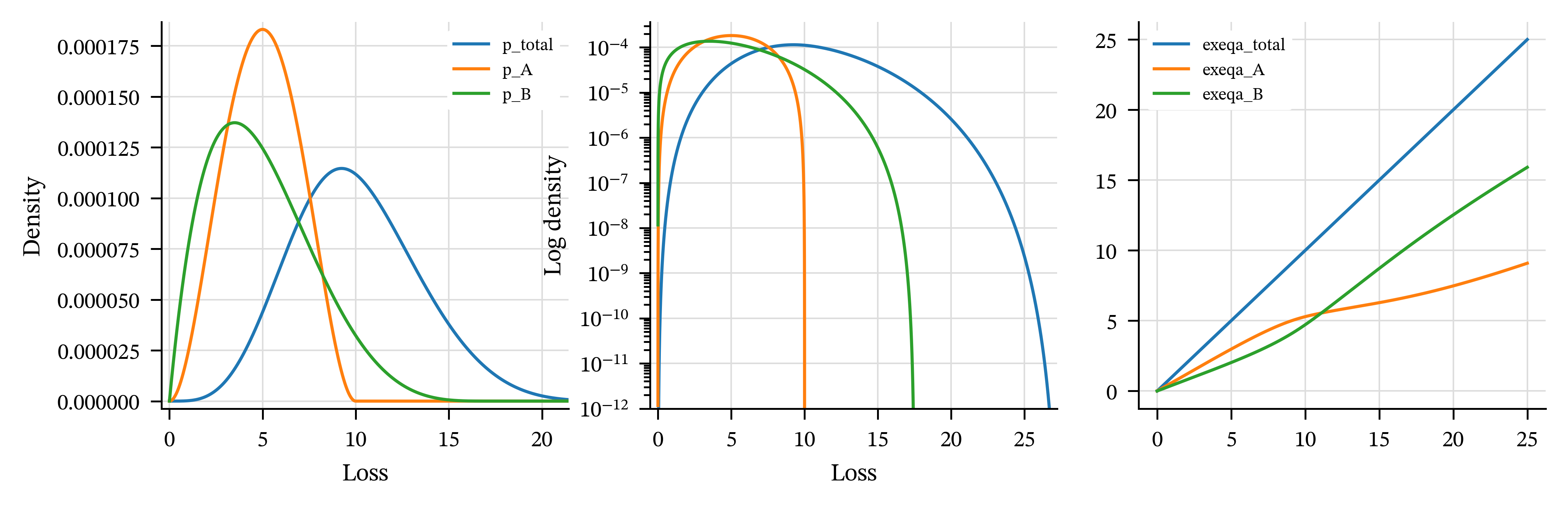
distortion	unit	L	P	M	Q	a	LR	PQ	COC
PH(0.537)	F	98.1	92.5	-5.63	1.29	93.8	106.1%	71.6	-435.1%
	V	3.13	12.5	9.38	18.7	31.2	25.0%	0.668	50.1%
	total	101	105	3.75	20	125	96.4%	5.25	18.8%

Example 4.23 (The Deniut–Roberts zone)

Table 4.24: CAPTION

distortion	unit	L	P	M	Q	a	LR	PQ	COC
PH(0.537)	F	98.1	92.5	-5.63	1.29	93.8	106.1%	71.6	-435.1%
	V	3.13	12.5	9.38	18.7	31.2	25.0%	0.668	50.1%
	total	101	105	3.75	20	125	96.4%	5.25	18.8%

Table 4.25: CAPTION

distortion	unit	L	P	M	Q	a	LR	PQ	COC
PH(0.537)	F	98.1	92.5	-5.63	1.29	93.8	106.1%	71.6	-435.1%
	V	3.13	12.5	9.38	18.7	31.2	25.0%	0.668	50.1%
	total	101	105	3.75	20	125	96.4%	5.25	18.8%

Example 4.24 (The Awkward zone)

Table 4.26: CAPTION

distortion	unit	L	P	M	Q	a	LR	PQ	COC
PH(0.537)	F	98.1	92.5	-5.63	1.29	93.8	106.1%	71.6	-435.1%
	V	3.13	12.5	9.38	18.7	31.2	25.0%	0.668	50.1%
	total	101	105	3.75	20	125	96.4%	5.25	18.8%

Table 4.27: CAPTION

distortion	unit	L	P	M	Q	a	LR	PQ	COC
PH(0.537)	F	98.1	92.5	-5.63	1.29	93.8	106.1%	71.6	-435.1%
	V	3.13	12.5	9.38	18.7	31.2	25.0%	0.668	50.1%
	total	101	105	3.75	20	125	96.4%	5.25	18.8%

4.9.5 Jordan Decomposition of Finite Variation Functions

This section recalls how to write a function of finite total variation as the difference of two increasing functions.

Let $f:[a,b]\to\mathbb{R}$ have finite (total) variation \[ V_a^b(f):=\sup_{\Pi}\sum_{i=1}^n |f(x_i)-f(x_{i-1})|<\infty, \] where the supremum is over partitions $\Pi: a=x_0<\cdots<x_n=b$.

Define the variation accumulated up to $x$ by \[ v(x)=V_a^x(f),\qquad x\in[a,b]. \]

The function $v$ is increasing, finite, and $v(a)=0$. For $a\le x<y\le b$, $ |f(y)-f(x)|V_x^y(f)=v(y)-v(x), $$ since, for any partition of $[x,y]$, the triangle inequality gives $|f(y)-f(x)|\le\sum|f(x_i)-f(x_{i-1})|$, and then take the supremum.

Define \[ f^+(x)=\frac{v(x)+f(x)-f(a)}{2},\qquad f^-(x)=\frac{v(x)-f(x)+f(a)}{2}. \] Then \[ f(x)=f(a)+f^+(x)-f^-(x), \tag{4.25}\] so $f$ is a difference of two increasing functions once we show $f^\pm$ are increasing.

To see the monotonicity of $f^+$: for $x<y$, \[ \begin{aligned} f^+(y)-f^+(x) &=\frac{v(y)-v(x)+f(y)-f(x)}{2} \\ &\ge \frac{v(y)-v(x)-|f(y)-f(x)|}{2} \\ \ge 0, \end{aligned} \] using step 2. Hence $f^+$ is increasing. Similarly, \[ \begin{aligned} f^-(y)-f^-(x) &=\frac{v(y)-v(x)-(f(y)-f(x))}{2} \\ &\ge \frac{v(y)-v(x)-|f(y)-f(x)|}{2} \\ &\ge 0, \end{aligned} \] so $f^-$ is increasing.

Equation eq-040-jordan is called thèJordan decomposition: any finite-variation $f$ equals a constant plus the difference of two increasing functions.

4.10 Advanced Properties of Distortions

posts/040-files/100-more-distortions.qmd

This section defines some properties of distortions that we use in sec-emergence. We start with some motivation in the context of a simple two-period pricing model.

Motivation. Consider a Bernoulli $s$ risk given explicitly by the random variable $X=\set{U<s}$ for a uniform $U$. Suppose $X$ becomes known at $t=2$, but that at $t=1$ we learn whether or not $U<\omega_I$ for some $\omega_I>s$. If $U<\omega_I$ holds, the risk $X$ becomes $X_I=\set{U<s\mid U<\omega_I}\sim \mathrm{Ber}(s/\omega_I)$, a Bernoulli with a higher probability of loss. If it does not hold, $X\equiv 0$. Use a SRM $g$ to price one-period risk transfer. Then at $t=1$ risk can be transferred for cost $g(s/\omega_I)$ in the first case, and for free in the second. This dichotomy creates a new random variable $V=g(s/\omega_I)\mathrm{Ber}(\omega_I)$ whose value is known at $t=1$. Applying $g$ to price $V$ gives it a price of $g(s/\omega_I)g(\omega_I)$, by positive homogeneity. Buying protection for $V$ transfers the two-period risk, acting like a replicating portfolio. The proceeds at $t=1$ are sufficient to buy a policy in the second period to transfer its risk. This idea, which we call P2P “policy to buy a policy” pricing is explored more in sec-050-p2p. Asking whether the P2P price $g(s/\omega_I)\mathrm{Ber}(\omega_I)$ is greater than or less than the single period price, $g(s)$, leads us to consider the multiplicative properties of $g$ \[ g(st)\ \stackrel{?}{\le}\ g(s)\,g(t). \]

4.10.1 Multiplicative Properties of Distortions

Definition 4.8 Let $h:[0,1]\to\mathbb R$ be a function.

$h$ is multiplicative function if $h(st)=h(s)h(t)$ for all $s,t\in[0,1]$.
$h$ is sub-multiplicative function if $h(st)\le h(s)h(t)$ for all $s,t\in[0,1]$.
$h$ is super-multiplicative function if $h(st)\ge h(s)h(t)$ for all $s,t\in[0,1]$.

Definition 4.9 Let $g:[0,1]\to[0,1]$ be a distortion function.

$g$ is multiplicative distortion if it is a multiplicative function.
$g$ is sub-multiplicative (SBM) distortion if it is a sub-multiplicative function.
$g$ is super-multiplicative (SPM) distortion if its dual $\check g$ is a super-multiplicative function.
$g$ is diagonal sub-multiplicative (DSBM) if it is sub-multiplicative along the diagonal, $g(s^2)\le g(s)^2$.

Notice the distinction between SBM which applies to $g$, and SPM which applies to $\check g$. If there is ambiguity we specify a sub- or super-multiplicative distortion or function. A distortion can be SBM and SPM, but if a function is both it must be multiplicative. Clearly SBM implies DSBM, but the converse is not true in general, though it does hold for BiTVaRs.

Define \[ h(s,t)=g(st)-g(s)g(t). \tag{4.26}\] In terms of $h$, SBM means $h\le 0$ on $[0,1]^2$, SPM means $h\ge 0$, and DSBM means $h(s,s)\le 0$ for all $s\in[0,1]$.

The next four lemmas describe the SBM and SPM behavior of common distortions. All proofs are gathered in sec-040-proofs, since they are largely technical or rely on ideas we yet to introduce.

Lemma 4.7

The mean distortion is multiplicative and hence SBM and SPM.
The max distortion SBM and SPM.
A proper $p$-TVaR distortion, $0<p<1$, is SBM but not SPM.
The CCoC distortion is SPM but not SBM.

Lemma 4.8 The proportional hazard distortion is SBM and SPM: it is a sub-multiplicative function and its dual is a super-multiplicative function.

Lemma 4.9 The Wang distortion is SBM and SPM: it is asub-multiplicative function and its dual is a super-multiplicative function.

Lemma 4.10 The dual distortion is SBM and SPM: it is a sub-multiplicative function and its dual is a super-multiplicative function.

Example 4.25 Theses lemmas might suggest that all differentiable distortions are SBM. This is not the case.

Add mixture examples.

There is no relationship between the SBM or SPM behavior of $g$ and its dual $\check g$. However, there is between $g$ and $g^{-1}$. Since $g$ may have flat spots, we have to define its inverse analogously to a quantile function, using the generalized inverse.

Definition 4.10 The generalized inverse of a distortion function $g$ (or an increasing function) is defined as \[ g^{-1}(u):=\inf\set{s\in[0,1]\mid g(s)\ge u},\qquad u\in[0,1]. \tag{4.27}\]

See Exercise exr-040-gen-inverse for some important properties of the generalized inverse.

Using the generalized inverse we can show that $g$ is a sub-multiplicativity function iff $g^{-1}$ is a super-multiplicativity function.

Lemma 4.11 A distortion function $g$ is SBM if and only if $g^{-1}$ is a SPM function.

4.10.2 Conditions for SBM and SPM

It is useful to translate the abstract conditions “$g$ is sub-multiplicative” and “$\check g$ is super-multiplicative” into concrete restrictions on how a distortion behaves. In general, these conditions are very subtle. However, it is possible to specify simple conditions that are quite powerful in special cases. One useful case is where $g$ is affine (a straight line) for sufficiently small $s$ or $s$ sufficiently close to $1$. The class of weighted TVaRs are affine near $0$ and $1$, which makes the next conditions useful.

Recall REF that any distortion can be represented as an integral weighting of TVaRs \[ g(s) = \int_{[0,1]} t_p(s)\,\nu(dp). \] The integral is a Lebesgue Stieltjes integral ($\nu$ can have jumps and does not necessarily have a density). In the case $\nu$ weights only finitely many points, call $g$ a weighted TVaR.

To help understand the next definition, consult Figure fig-corner-conditions.

Definition 4.11 Let $g$ be a distortion with TVaR measure $\nu$.

$g$ weights the max if $\nu\set{1}>0$.
$g$ weights the mean if $\nu\set{0}>0$.
If $g$ weights the max and $0<\nu\set{1}<1$ we say $g$ has property $M$.
If $g$ weights the mean and is eventually linear as $s\uparrow 1$ we say $g$ has property $S$.
If $g$ does not weight the mean and is eventually linear as $s\uparrow 1$ and $\nu\set{1}<1$ we say $g$ has property $\check M$.
If $g$ does not weight the max and is eventually linear as $s\downarrow 0$ we say $g$ has property $\check S$.

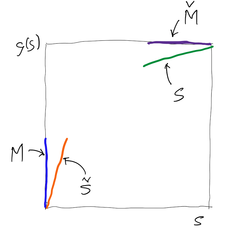
Figure 4.10: Two pairs of distortion corner condition behavior: $M$ and $\check M$, and $\check S$ and $S$.

The notation reflects that $M$ and $\check M$ are dual conditions, as are $S$ and $\check S$.

If $g$ has property $M$, then $g(0+):=\lim_{s\downarrow 0}g(s)>0$ and $g$ is not continuous at $0$. Property $\check S$ means there are $\epsilon,\,k>0$ so that $g(s)=ks$ for $s<\epsilon$. Jouini et al. (2008) calls this property “eventually risk neutral”. These two properties are mutually exclusive and describe behavior near $s=0$.

If $g$ has property $S$, then $g'(1-)<1$ and there are $\epsilon>0$ and $0<k<1$ so that $g(s) = kx + 1-k$ is affine with slope $k$ through $(1,1)$. If $g$ has property $\check M$, it ends with a “flat interval” and there is $\epsilon>0$ so that $g(s)=1$ for $s>1-\epsilon$. These two properties are also mutually exclusive and describe behavior near $s=1$. They can coexist with either $M$ or $\check S$.

All weighted TVaRs are either $M$ or $\check S$, and either $\check M$ or $S$. However, other distortions have none of these four properties: for example none applies to the PH, Wang, or dual. The PH weights the mean, but is not affine as it approaches $1$. See Remark rem-040-tail-behavior for a discussion of what happens when the affine assumption does not hold.

The four properties us to rule out certain behaviors very easily, and, in particular, help to characterize when a biTVaR is SMB or SPM.

Lemma 4.12 Let $g$ be a distortion. Then

If $M$ then $g$ is not sub-multiplicative. Conversely, if $g$ is SBM then it is continuous.
If $\check M$ then $\check g$ is not super-multiplicative.
If $S$ then $g$ is not sub-multiplicative.
If $\check S$ then $\check g$ is not super-multiplicative.

Proof. We give the proof here because it is quite instructive.

If $M$, then $g(0+)=\lim_{s\downarrow 0} g(s)=\epsilon>0$ and $\epsilon < 1$. For small $s$, $g(s)\approx \epsilon$ and $g(s^2)\approx \epsilon$ but $g(s)^2\approx \epsilon^2<\epsilon$ (using $\epsilon < 1$), showing $g$ is not DSBM and hence not SBM. Thus, SBM $\Rightarrow g(0+)=0$.
If $\check M$, then there exists $s_0<1$ so that $g(s)=1$ for all $s\ge s_0$. This makes the dual distortion equal to zero for small $s$ and hence it cannot be super-multiplicative: take $u,v>1-s_0$ so that $uv<1-s_0$, then $\check g(uv)=0 < \check g(u)\check g(v)$. We need the mass at the max to be $<1$ to find points $u$ with $\check g(u)>0$.
If $S$, then sufficiently close to $s=1$ we can write $g(s)=1 + k(s-1)=1-k + ks$, for $s>s_0$ and $k<1$. Since we are interested in the behavior near $s=1$, write $s=1-t$ and assume that $t$ is sufficiently small that $1-t> (1-t)^2 > s_0$. Then, $g(1-t)= (1-k)+k(1-t) = 1-kt$ showing $g(1-t)^2=(1-kt)^2=1-2kt+k^2t^2$. On the other hand, $g((1-t)^2)=(1-k)+k(1-2t+t^2)=1-2kt+kt^2$. But then $g(1-t)^2-g((1-t)^2)= 1-2kt+k^2t^2 - (1-2kt+kt^2)= -kt^2(1-k)<0$ since $k<1$. Therefore $g(s)^2<g(s^2)$, showing that $g$ is not sub-multiplicative.
If $\check S$, then sufficiently close to $s=1$ we can write $\check g(s)=1 + k(s-1)=1-k + ks$, for $s>s_0$ and $k>1$ (draw a picture). Since we are interested in the behavior near $s=1$, write $s=1-t$ and assume that $t$ is sufficiently small that $1-t> (1-t)^2 > s_0$. Then, $\check g(1-t)= (1-k)+k(1-t) = 1-kt$ showing $\check g(1-t)^2=(1-kt)^2=1-2kt+k^2t^2$. On the other hand, $\check g((1-t)^2)=(1-k)+k(1-2t+t^2)=1-2kt+kt^2$. But then $\check g(1-t)^2-\check g((1-t)^2)= 1-2kt+k^2t^2 - (1-2kt+kt^2)= kt^2(k-1)>0$ since $k>1$. Therefore $\check g(s^2)<\check g(s)^2$, showing that $\check g$ is not super-multiplicative.

Lemma lem-sub-super implies that the absence of both sub- and super-multiplicative behavior can be determined from $S/\check S$ or $M/\check M$ but the mixed cases $S/M$ (resp. $\check S/\check M$) both relate to sub-multiplicative (super-multiplicative) behavior and are not dispositive. Table tbl-bitvar-sub-super shows how the conditions pair up, with two useful pairs and two not useful.

Table 4.28: Sub- and super-multiplicative behavior distortions, with common examples.

Quality	Symbol	Weights Max	Does not wt max, affine
		$M$	$\check S$
Weights mean, affine	$S$	Not sub, maybe super	Neither sub nor super
Examples		CCoC	Mean-BiTVaR

Does not wt mean	$\check M$	Neither sub nor super	Not super, maybe sub
Examples		Max-BiTVaR	BiTVaR

4.10.3 BiTVaRs

Definition 4.12 A BiTVaR distortion is a convex combination of two TVaR distortions: \[ g(s)=w\,\mathsf{TVaR}_{p_0}(s) + (1-w)\,\mathsf{TVaR}_{p_1}(s), \qquad 0<p_0<p_1<1,\quad 0<w<1. \] We call the BiTVaR proper if all weights satisfy $0<w<1$ and $0<p_0<p_1<1$, otherwise it is degenerate.

A proper TVaR corresponds to a degenerate BiTVaR with a single $p$, $0<p<1$. The CCoC, mean, and max are all degenerate BiTVaRs. For a proper BiTVaR, fix $0<p_0<p_1<1$ and weights $w\in(0,1)$, $1-w$, and define the kink points (?kink) \[ s_0:=1-p_0,\qquad s_1:=1-p_1, \qquad 1>s_0>s_1>0. \] The distortion function has exactly three affine pieces: \[ g(s)= \begin{cases} m_0\,s, & 0\le s\le s_1,\\ b+m_1\,s, & s_1<s\le s_0,\\ 1, & s_0<s\le 1, \end{cases} \] where \[ m_1:=\frac{w}{s_0},\qquad b:=1-w,\qquad m_0:=m_1+\frac{1-w}{s_1}=\frac{w}{s_0}+\frac{1-w}{s_1}. \]

In general there are eight types of BiTVaR, laid out in Table tbl-bitvar-sub-super-2 and illustrated in Figure fig-bitvar-sub-super-01. The box color column in the table references the figure.) Figure fig-bitvar-sub-super-grid shows representative shapes for each type. Only the two bottom rows of the table are proper, the rest degenerate. In the figure, the box color corresponds to the symbol in the upper left-hand corner of each plot. The table is in the same order as the graphic, left-to-right, top-to-bottom. Throughout the table $p_0<p_1$, unless otherwise specified. Looking at the right-hand part of the figure:

Distortions in the left vertical orange box have $p_0=0$ and weight the mean, giving $S$ and so are not SBM, and $p_1>0$ giving $\check S$ and so not SPM.
Those in the horizontal top purple box have $p_1=1$ and weight the max, giving $M$ and so are not SPM, and $p_0>0$ so the mean is not weighted giving $\check M$ and so not SPM.

Figure 4.11: Sub- and super-multiplicative properties of BiTVaRs.

Figure 4.12: Sub- and super-multiplicative properties of BiTVaRs.

Table 4.29: The eight types of BiTVaR distortions and their extreme point behavior at $s=0$ and $s=1$, and their SBM and SPM behavior.

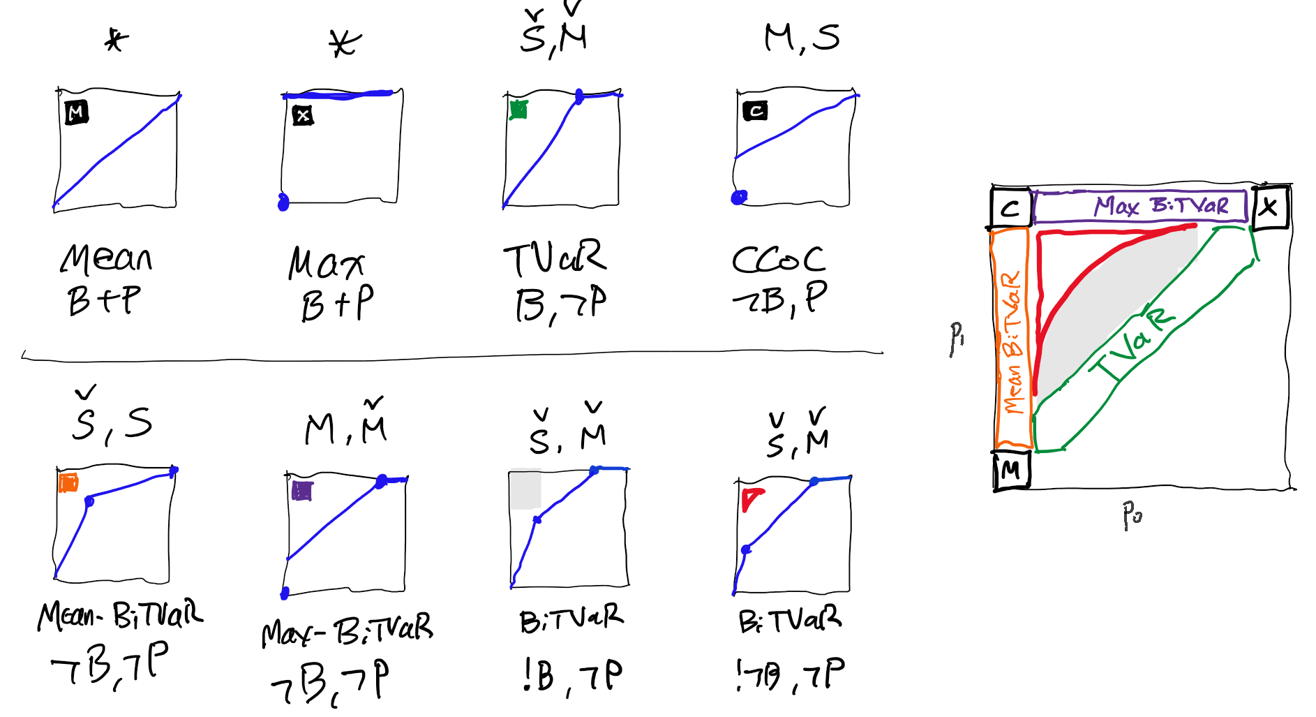
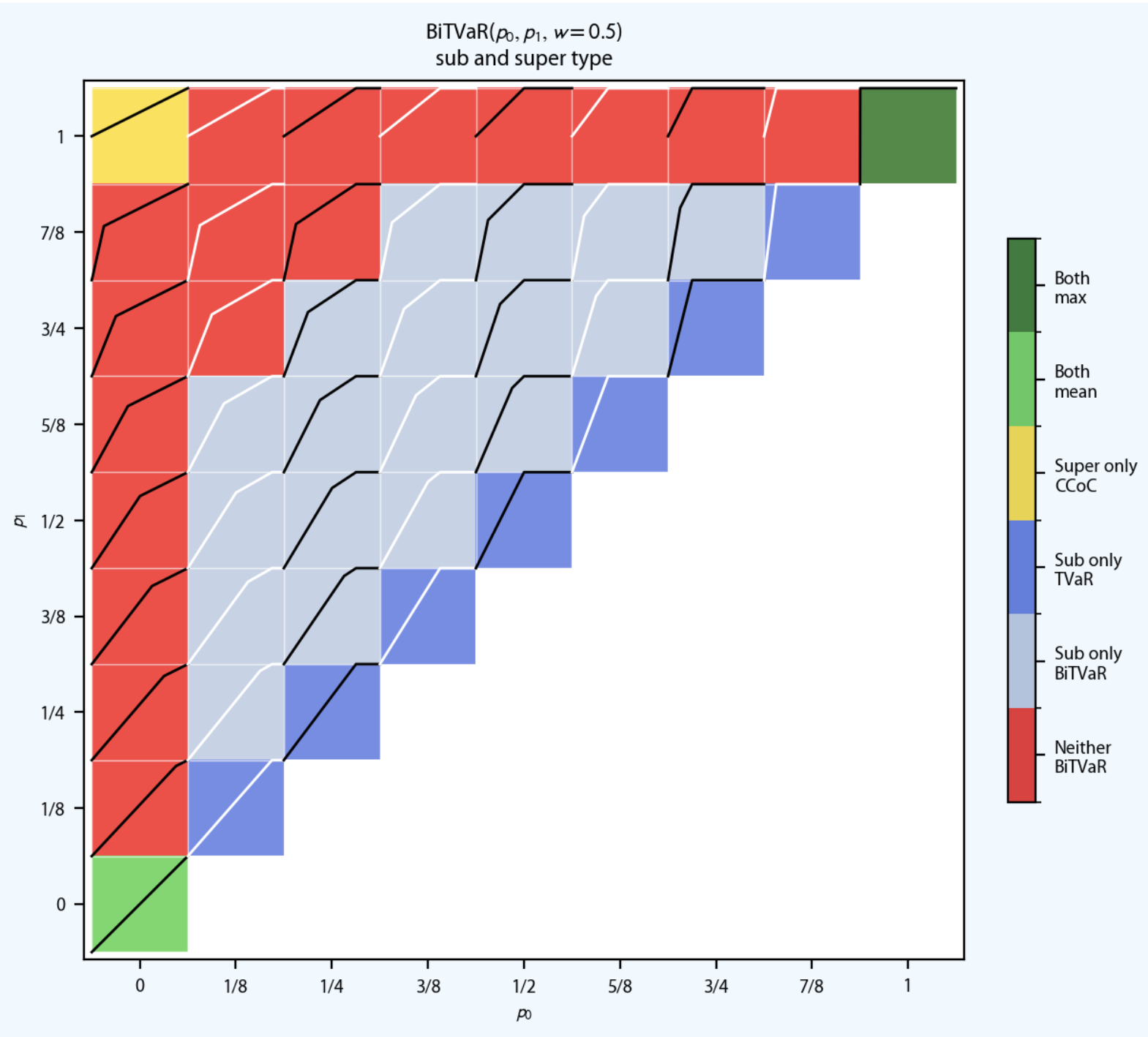
Name	Low $p_0$	High $p_1$	$s=0$	$s=1$	SBM	SPM	Box Color
Mean	$p_0=0$	$p_1=0$	n/a${}^{1}$	n/a${}^{1}$	Yes$^{\,2}$	Yes$^{\,2}$	Black M
Max	$p_0=1$	$p_1=1$	n/a${}^{10}$	n/a${}^{10}$	Yes$^{\,9}$	Yes$^{\,9}$	Black X
TVaR	$p_0>0$	$p_1=p_0<1$	$\check S$	$\check M$	Yes$^{\,8}$	No$^{\,4,7}$	Green
CCoC	$p_0=0$	$p_1=1$	$M$	$S$	No$^{\,3,5}$	Yes$^{\,6}$	Black C
Mean-BiTVaR	$p_0=0$	$p_1<1$	$\check S$	$S$	No$^{\,3}$	No$^{\,4}$	Orange
Max-BiTVaR	$p_0>0$	$p_1=1$	$M$	$\check M$	No$^{\,5}$	No$^{\,7}$	Purple
BiTVaR$_{b}$	$p_0>0$	$p_1<1$	$\check S$	$\check M$	Yes$^{\,11}$	No$^{\,4,7}$	Grey
BiTVaR	$p_0>0$	$p_1<1$	$\check S$	$\check M$	No$^{\,11}$	No$^{\,4,7}$	Red

Notes to Table tbl-bitvar-sub-super-2.

Neither $\check S$ nor $S$ because that requires slope $\not=1$.
The mean is obviously multiplicative, and hence sub- and super-multiplicative. Relies on slope $1$.
$S$ is not sub-multiplicative.
$\check S$ is not super-multiplicative.
$M$ is not sub-multiplicative.
CCoC is SPM by Lemma lem-040-basic-sub-super.
$\check M$ is not super-multiplicative.
TVaR is SBM by Lemma lem-040-basic-sub-super.
The max is trivially multiplicative, and hence sub- and super-multiplicative.
Max is neither $M$ nor $\check M$ because $\nu\set{1}=1$.
The distinguishing condition between the last two rows is stated and proved in Proposition prp-sub-super-bitvar.

Lemma lem-040-basic-sub-super proves the claims in the first six rows of Table tbl-bitvar-sub-super-2, but it cannot be extended to determine the behavior of the proper BiTVaRs in the last two, because it is more subtle. They are never SPM but may be SBM under certain conditions. To see that, it is helpful to start by observing that for BiTVaRs DSBM implies SBM, which is a helpful simplification.

Proposition 4.8 A continuous biTVaR distortion $g$ is SBM if and only if it is DSBM.

We can now characterize the two types of proper BiTVaRs.

Proposition 4.9 Let $g$ be a proper BiTVaR defined by $0 < p_0 < p_1<1$ weighting $p_1$ by $0 < w < 1$. Then $g$ is sub-multiplicative if and only if \[ g(s_1)\le g(\sqrt{s_1})^2, \] and this condition holds if and only if $s_0\le s_0(s_1)$, where $s_0(s_1)$ is the positive root of \[ w s_0^2 + s_0\bigl(s_1-2w\sqrt{s_1}\bigr) - (1-w)s_1 = 0. \]

4.10.4 Algorithm to determine $\max h$ for a Weighted TVaR

In this section we extend the ideas in the proofs of Proposition prp-040-DSBM-bitvars and Proposition prp-sub-super-bitvar to give an algorithm to determine the maximum value of $h(u,v)=g(uv)-g(u)g(v)$ for a general continuous weighted TVaR $g$. The function $g$ is a piecewise-linear function and it can be represented by its kinks \[ 0=x_0<x_1<\cdots<x_n=1, \qquad y_r=g(x_r). \] On each segment $[x_r,x_{r+1}]$, \[ g(u)=m_r u + b_r, \qquad m_r=\frac{y_{r+1}-y_r}{x_{r+1}-x_r}, \qquad b_r=y_r-m_r x_r. \]

The goal is to compute \[ h_{\max}=\max_{(s,t)\in[0,1]^2} h(s,t) \] exactly, by evaluating $h$ on a finite candidate set.

Algorithm `ExactMaxMultiplicativityExcess(g)`

Inputs:

kinks x[0..n], values y[0..n], with x[0]=0, x[n]=1
$g$ is continuous piecewise-linear by linear interpolation of $(x,y)$

Outputs:

h_max and a maximizer (s_max,t_max)

Precompute:

For r=0..n-1:
   m[r] = (y[r+1]-y[r])/(x[r+1]-x[r])
   b[r] = y[r]-m[r]\*x[r]

Define Seg(u): segment index of u
   Seg(u) := largest r with x[r] <= u < x[r+1], clipped into {0,...,n-1}
   (take Seg(1)=n-1)

Candidate set C := empty set

Step A: gather kink-grid points (rectangle corners)

   For each i in {0,...,n}:
     For each j in {0,...,n}:
        add (x[i], x[j]) to C

Step B: hyperbola endpoints inside kink-rectangles

   For each kink value c in {x[1],...,x[n]} with c>0:
      For each i in {1,...,n} with x[i]>0:
        add (x[i], c/x[i]) to C   (if in [0,1]^2)
     For each j in {1,...,n} with x[j]>0:
        add (c/x[j], x[j]) to C   (if in [0,1]^2)

Step C: stationary points on hyperbola arcs st=c

   For each kink value c in {x[1],...,x[n]} with c>0:
     For each s-segment index i in {0,...,n-1}:
       For each t-segment index j in {0,...,n-1}:

         Consider the arc domain where
           s in [x[i], x[i+1]],
           t = c/s in [x[j], x[j+1]].

         Compute stationary point candidate (if it exists):
           Require m[i]>0, b[i]>0, m[j]>0, b[j]>0.
           q = (m[j]\*b[i]\*c)/(m[i]\*b[j]).
           If q <= 0: continue.
           s_star = sqrt(q), t_star = c/s_star.

         Feasibility test:
           If s_star in [x[i],x[i+1]] AND t_star in [x[j],x[j+1]]:
              add (s_star, t_star) to C

Evaluate

   For each (s,t) in C:
     compute h(s,t)=g(st)-g(s)g(t)
   Return the maximum value and its argmax.

Step A covers all kink-rectangle corners, including axes intersections. Step B covers endpoints of hyperbola arcs where $st=c$ crosses vertical or horizontal kink lines. Step C covers the only possible interior extrema of $h$ restricted to a hyperbola boundary. The candidate set is finite and typically small enough to evaluate quickly, even for hundreds of kinks.

4.10.5 TriTVaRs

Example 4.26 (TriTVaR that is DSBM but not SBM) For BiTVaR, DSBM is equivalent to SBM. But for TriTVaR the two are distinct, as this example shows.

EXAMPLE.

4.10.6 Elasticity

Definition 4.13 The elasticity function $\eta:[0,1]\to[0,1]$ associated with a distortion $g$ is \[ \eta(s) = \frac{sg'(s)}{g(s)} \] where $g$ is differentiable. The left (minus) and right (plus) elasticity are defined for all $s$ by \[ \eta^\pm(s) = \frac{sD^\pm g(s)}{g(s)} \] where \[ D^\pm g(x)= \lim_{\epsilon\downarrow 0} \frac{g(x\pm \epsilon) - g(x)}{\pm \epsilon} \] are the left and right derivatives.

See Simon (2011) for details on the left and right derivatives. They always exist and both equal the standard derivative when it exists. The left derivative is $\le$ the right.

Elasticity $\eta(s)\ge 0$ since all its ingredients are $\ge 0$. Since $g$ is concave, $g'(s) \le g(s) / s$ with equality before the first kink of a weighted TVaR, for example. Hence $\eta(s)\le 1$.

Elasticity measures the marginal percent change in price per percent change in probability. In the Bernoulli setting, $\eta$ summarizes how the pricing rule treats small shifts in loss probability.

Two endpoint regimes matter. It $\eta(0)=0$, then marginal risk is cheap for large losses. This occurs when $g(0+)>0$ (a fixed-cost or minimum-premium component). CCoC has $\eta(0)=0$ because $g(s)=d+vs$ has a fixed-cost term $d>0$. In addition, many smooth concave distortions used in practice behave like $\eta(s)\to 0$ as $s\downarrow 0$, including concave proportional hazards and Wang. When $\eta(0)=0$, increasing the conditional probability of loss from small $s$ to a slightly larger $s_\omega$ is relatively inexpensive, because the marginal cost is low compared to the existing price level. This has implications for P2P pricing, see REF.

At the other extreme, if $\eta(0)=1$ then marginal risk is not discounted at the origin. For distortions with $g(s)\sim c s$ as $s\downarrow 0$ (or affine near $0$), we has $\eta(s)\to 1$. This includes $p$ TVaR for $s<1-p$ and the dual power family near $0$. When $\eta(0)=1$, increasing loss probability is not “cheap” in relative terms: small increases in $s$ translate proportionally into increases in $g(s)$.

4.10.7 Properties of the Representative Distortions

TODO Make Table

Plot $g$, $g'(1-s)$, $-(1-p)g''(1-p)=\nu$, $\eta(s)=s'g(s) / g(s)$, loss ratio, loss to asset leverage, discount $(g(s)-s) / (1 - s)$
Table of $g'(0+)$, $g'(1-)$, SBM, SPM, etc.

Remark 4.16 (Behavior of the Wang at $s=0,1$.). Let \[ g_\lambda(s)=\Phi(\Phi^{-1}(s)+\lambda),\qquad 0<s<1, \] be the Wang distortion and set $z=\Phi^{-1}(s)$. Then $dz/ds=1/\phi(z)$, so \[ g_\lambda'(s)=\phi(z+\lambda)\frac{1}{\phi(z)}=\frac{\phi(z+\lambda)}{\phi(z)} =\exp\!\left(-\lambda z-\frac{\lambda^2}{2}\right). \] Now take limits at the endpoints.

As $s\downarrow 0$, $z=\Phi^{-1}(s)\to -\infty$, hence \[ g_\lambda'(0+)=\lim_{z\to-\infty}\exp\!\left(-\lambda z-\frac{\lambda^2}{2}\right) = \begin{cases} +\infty, & \lambda>0,\\ 1, & \lambda=0,\\ 0, & \lambda<0. \end{cases} \]

As $s\uparrow 1$, $z=\Phi^{-1}(s)\to +\infty$, hence \[ g_\lambda'(1-)=\lim_{z\to+\infty}\exp\!\left(-\lambda z-\frac{\lambda^2}{2}\right) = \begin{cases} 0, & \lambda>0,\\ 1, & \lambda=0,\\ +\infty, & \lambda<0. \end{cases} \]

4.10.8 Proofs

This section presents proofs of results from in sec-040-100.

Proof (Of Lemma lem-040-basic-sub-super). We use Lemma lem-sub-super for claims involving $M$ and $\check M$

Obvious.
Obvious.
The TVaR$_p$ distortion is given by $g(s)=\displaystyle\frac{s}{1-p}\wedge 1$. It is not super-multiplicative because it is $\check M$. To see it is sub-multiplicative, consider four exhaustive cases where we can assume $s<t$:
- if $t \le 1-p$, then $g(st)= \displaystyle\frac{st}{1-p} \le \displaystyle\frac{s}{1-p}\displaystyle\frac{t}{1-p}=g(s)g(t)$ because $1-p<1$;
- if $s\le 1-p < t \le 1$, then $g(t)=1$ and $g(st) = \displaystyle\frac{st}{1-p} \le \displaystyle\frac{s}{1-p}= g(s)g(t)$;
- if $st \le 1-p < s$, then $g(st) = \displaystyle\frac{st}{1-p} < 1 = g(s)g(t)$; and finally
- if $1-p \le st$, then $g(st) = 1= g(s)g(t)$.
CCoC is not sub-multiplicative because it is $M$. To see it is super-multiplicative, first note $\check g(s)=1-g(1-s)=1-(d + v(1-s))=vs$ if $s<1$ and $\check g(1)=1$. super-multiplicativity now follows because $v<1$. If $s,t<1$ then $\check g(st)=vst > v^2st = \check g(s)\check g(t)$. If $t=1$, $\check g(st)=vs = \check g(s)\check g(t)$.

REVIEW - WRONG AS STATED - LOOK AT INEQUALITY APPLIED!

Exercise 4.8 Let $g:[0,1]\to[0,1]$ be a distortion function: nondecreasing, with $g(0)=0$, $g(1)=1$, and right-continuous on $[0,1)$. Define its generalized inverse by Equation eq-040-gen-inv-def. Prove the following.

$g^{-1}$ is nondecreasing.
For $x,y\in[0,1]$ we have \[ y \le g(x)\iff g^{-1}(y)\le x. \tag{4.28}\]
$g(g^{-1}(y))\ge y$ for all $y\in[0,1]$.
$g^{-1}(g(x))\le x$ for all $x\in[0,1]$.
It is not true in general that \[ g(x)\le y \iff x\le g^{-1}(y). \]

Solution 4.7. Let $A_y:=\{s\in[0,1]:g(s)\ge y\}$, so $g^{-1}(y)=\inf A_y$. Since $g(1)=1$, we have $A_y\neq\varnothing$ for all $y\in[0,1]$.

If $u\le v$, then $A_v\subseteq A_u$. Taking the infimum gives \[ g^{-1}(u)=\inf A_u\le \inf A_v=g^{-1}(v), \] so $g^{-1}$ is nondecreasing.
($\implies$) If $y\le g(x)$, then $x\in A_y$, hence $\inf A_y\le x$, i.e. $g^{-1}(y)\le x$.

($\impliedby$) Let $\alpha:=g^{-1}(y)=\inf A_y$ and assume $\alpha\le x$. By the definition of infimum, for each $n\ge1$ there exists $s_n\in A_y$ with \[ \alpha\le s_n<\alpha+\frac1n. \] Then $s_n\downarrow \alpha$ and $g(s_n)\ge y$ for all $n$. Since $g$ is nondecreasing, $g(s_n)\downarrow g(\alpha+)$. Right-continuity at $\alpha$ yields $g(\alpha+)=g(\alpha)$, hence \[ g(\alpha)=\lim_{n\to\infty}g(s_n)\ge y. \] Monotonicity and $\alpha\le x$ give $g(x)\ge g(\alpha)\ge y$, so $y\le g(x)$.
Let $\alpha:=g^{-1}(y)$. By the same construction as in (2), there exists $s_n\downarrow \alpha$ with $s_n\in A_y$, hence $g(s_n)\ge y$ for all $n$. As above, $g(s_n)\downarrow g(\alpha+)=g(\alpha)$ by right-continuity at $\alpha$, so \[ g(g^{-1}(y))=g(\alpha)=\lim_{n\to\infty}g(s_n)\ge y. \]
Let $x\in[0,1]$ and set $y:=g(x)$. Then $x\in A_y$ because $g(x)\ge y$. Therefore \[ g^{-1}(g(x))=g^{-1}(y)=\inf A_y\le x. \]
Suppose $g$ is flat on $[x_0,x_1]$ with $0\le x_0<x_1\le1$, and set $y:=g(x_0)=g(x_1)$. Then $g(x_1)\le y$ holds, but \[ g^{-1}(y)=\inf\{s:g(s)\ge y\}=x_0, \] so $x_1\le g^{-1}(y)$ is false. Hence $g(x)\le y\implies x\le g^{-1}(y)$ fails in general, and therefore the displayed bi-implication is not true in general.

Proof (Of Lemma lem-040-inverse). Assume $g$ is sub-multiplicative. Let $u,v\in[0,1]$ and set $s=g^{-1}(u)$, $t=g^{-1}(v)$. Then by Equation eq-040-gen-inv, \[ g(s)\le u,\qquad g(t)\le v, \] so \[ g(st)\le g(s)g(t)\le uv. \] Applying Equation eq-040-gen-inv again gives \[ st \le g^{-1}(uv), \] i.e. \[ g^{-1}(uv)\ge g^{-1}(u)\,g^{-1}(v). \] So $g^{-1}$ is super-multiplicative.

Conversely, assume $g^{-1}$ is super-multiplicative. Take any $s,t\in[0,1]$ and put $u=g(s)$, $v=g(t)$. Then $s\le g^{-1}(u)$ and $t\le g^{-1}(v)$, giving \[ g^{-1}(u)\,g^{-1}(v)\ge st. \] By super-multiplicativity, \[ g^{-1}(uv)\ge g^{-1}(u)\,g^{-1}(v)\ge st. \] Applying $g$ (monotone) yields \[ g\!\left(g^{-1}(uv)\right)\ge g(st). \] But $g(g^{-1}(y)) \ge y$ for all $y$, so $g(st) \ge uv = g(s)g(t)$ and so $g$ is super-multiplicative.

The next lemma provides a handy trick for converting SBM/SPM into sub- or super-additivity.

Lemma 4.13 Let $u(x)=\log g(e^x)$ for $x\le 0$. Then $g$ is sub-multiplicative if and only if $u$ is subadditive \[ u(x+y)\le u(x)+u(y)\qquad(x,y\le 0). \]

Proof. Take $s=e^x$, $t=e^y$.

Proof (Proof of Lemma lem-040-ph-sub-super-rep). The PH is multiplicative and hence SBM and a SPM function. The dual is $\check g(s)= 1 - (1-s)^a$ with $0\le a\le 1$ (note the dual distortion requires exponent $b\ge 1$.) FINISH UP.

Proof (Proof of Lemma lem-040-dual-sub-super-rep). Let $m>1$ and define the dual power distortion \[ g(s)=1-(1-s)^m,\qquad s\in[0,1]. \] We prove $g$ is sub-multiplicative: \[ g(st)\le g(s)g(t)\qquad\forall s,t\in[0,1]. \]

Set $a=1-s$ and $b=1-t$, so $a,b\in[0,1]$ and \[ 1-st = 1-(1-a)(1-b)=a+b-ab. \] Then \[ g(st)=1-(1-st)^m = 1-(a+b-ab)^m, \] and \[ g(s)g(t) = \bigl(1-a^m\bigr)\bigl(1-b^m\bigr)=1-a^m-b^m+(ab)^m. \] Therefore $g(st)\le g(s)g(t)$ is equivalent to \[ 1-(a+b-ab)^m \le 1-a^m-b^m+(ab)^m, \] i.e. \[ (a+b-ab)^m + (ab)^m \ge a^m + b^m. \tag{1} \]

Let $S=a+b$ and define \[ h(x)=x^m + (S-x)^m,\qquad x\in[0,S]. \] Since $m>1$, $x\mapsto x^m$ is convex on $[0,\infty)$, so $h$ is convex on $[0,S]$ and symmetric about $S/2$: \[ h(x)=h(S-x). \] Also, \[ a^m+b^m = a^m+(S-a)^m = h(a), \] and \[ (a+b-ab)^m+(ab)^m = (S-ab)^m + (ab)^m = h(S-ab). \] So (1) becomes \[ h(S-ab)\ge h(a). \tag{2} \]

Assume without loss of generality that $a\ge b$. Then $a\ge S/2$. Moreover, \[ (S-ab)-a = (a+b-ab)-a = b(1-a)\ge 0, \] so \[ S-ab \ge a \ge S/2. \] For $x\in[S/2,S]$ we have \[ h'(x)=m\bigl(x^{m-1}-(S-x)^{m-1}\bigr)\ge 0, \] so $h$ is nondecreasing on $[S/2,S]$. Hence, from $S-ab\ge a\ge S/2$, \[ h(S-ab)\ge h(a), \] which is (2), hence (1), hence $g(st)\le g(s)g(t)$.

Therefore $g(s)=1-(1-s)^m$ is sub-multiplicative for every $m>1$.

Proof (Proof of Lemma lem-040-wang-sub-super-rep.). Fix $\lambda \ge 0$ and define the Wang distortion \[ g_\lambda(s) = \Phi(\Phi^{-1}(s)+\lambda), \qquad 0\le s\le 1, \] where $\Phi$ and $\phi$ are the standard normal CDF and density.

First, note that the dual of $g_\lambda$ is just a Wang with parameter $-\lambda$. By definition, $\check g_\lambda(s)=1-g_\lambda(1-s)$. Using $\Phi^{-1}(1-s)=-\Phi^{-1}(s)$ and $1-\Phi(x)=\Phi(-x)$, \[ \begin{aligned} \check g_\lambda(s) &=1-\Phi(\Phi^{-1}(1-s)+\lambda) \\ &=1-\Phi(-\Phi^{-1}(s)+\lambda) \\ &=\Phi(\Phi^{-1}(s)-\lambda) \\ &=g_{-\lambda}(s). \end{aligned} \] So for $\lambda\ge 0$, the dual of $g_\lambda$ is $g_{-\lambda}$ with a nonpositive parameter.

We must show that if $\lambda\ge 0$, then $g_\lambda(uv)\le g_\lambda(u)\,g_\lambda(v)$ (sub-multiplicative), and if $\lambda\le 0$, then $g_\lambda(uv)\ge g_\lambda(u)\,g_\lambda(v)$ (super-multiplicative). In particular, for $\lambda\ge 0$, the dual $\check g_\lambda=g_{-\lambda}$ is super-multiplicative.

Assume $u,v\in(0,1]$. For $s\in(0,1]$ and $x\ge 0$, define \[ r_\lambda(s)=\frac{g_\lambda(s)}{s}, \quad\text{and}\quad \psi_\lambda(x)=\log r_\lambda(e^{-x}). \] Then $r_\lambda(1)=1$ so $\psi_\lambda(0)=0$, and \[ \begin{aligned} g_\lambda(uv)\le & (\ge)\, g_\lambda(u)g_\lambda(v) \\ \iff r_\lambda(uv)\le & (\ge)\, r_\lambda(u)r_\lambda(v) \\ \iff \psi_\lambda(x+y)\le & (\ge)\, \psi_\lambda(x)+\psi_\lambda(y), \end{aligned} \] with $u=e^{-x}$ and $v=e^{-y}$.

We use two elementary facts about functions on $\mathbb R_+$ with value $0$ at $0$. First, if $\psi$ is concave and $\psi(0)=0$, then $\psi(x+y)\le \psi(x)+\psi(y)$. To see this, apply concavity to $x = (x/(x+y))(x+y) + (y/(x+y))0$ and similarly for $y$ and add the two inequalities. Second, if $\psi$ is convex and $\psi(0)=0$, then $\psi(x+y)\ge \psi(x)+\psi(y)$ by applying the concavity result to $-\psi$.

Therefore it suffices to show: $\psi_\lambda$ is concave for $\lambda\ge 0$ and convex for $\lambda\le 0$.

Now set $t=t(x)=\Phi^{-1}(e^{-x})$, so $e^{-x}=\Phi(t)$ and $x=-\log\Phi(t)$. Define the inverse Mills ratio \[ m(t)=\frac{\phi(t)}{\Phi(t)}. \] Then \[ \psi_\lambda(x)=\log\left(\frac{\Phi(t+\lambda)}{\Phi(t)}\right) =\log\Phi(t+\lambda)-\log\Phi(t), \] and \[ \frac{dx}{dt}=-m(t), \qquad \frac{dt}{dx}=-\frac{1}{m(t)}. \] Differentiate: \[ \psi_\lambda'(x) =\left(m(t+\lambda)-m(t)\right)\frac{dt}{dx} =1-\frac{m(t+\lambda)}{m(t)}. \] Differentiate again (using $d/dx=(dt/dx)\,d/dt$): \[ \psi_\lambda''(x) =\frac{m(t)m'(t+\lambda)-m(t+\lambda)m'(t)}{m(t)^3}. \] Hence $\operatorname{sign}(\psi_\lambda'')$ is the sign of \[ m(t)m'(t+\lambda)-m(t+\lambda)m'(t), \] which is nonpositive exactly when the log-derivative $m'(t)/m(t)$ is decreasing.

The identity \[ m'(t)=-m(t)\,(t+m(t)) \] is standard for the inverse Mills ratio. So \[ \frac{m'(t)}{m(t)}=-(t+m(t)). \] Therefore $m'(t)/m(t)$ is decreasing if and only if $t+m(t)$ is increasing.

To see that $t+m(t)$ is increasing, differentiate: \[ \frac{d}{dt}\bigl(t+m(t)\bigr)=1+m'(t)=1-t\,m(t)-m(t)^2. \] But for $Z\sim N(0,1)$, the one-sided truncated normal variance satisfies \[ \mathsf{var}(Z\mid Z\le t)=1-t\,\frac{\phi(t)}{\Phi(t)}-\left(\frac{\phi(t)}{\Phi(t)}\right)^2, \] so $1-t\,m(t)-m(t)^2=\mathsf{var}(Z\mid Z\le t)>0$. Thus $t+m(t)$ is strictly increasing, so $m'(t)/m(t)$ is strictly decreasing.

Now compare $t+\lambda$ to $t$. If $\lambda\ge 0$, then $t+\lambda\ge t$ and decreasing of $m'/m$ gives \[ \frac{m'(t+\lambda)}{m(t+\lambda)}\le \frac{m'(t)}{m(t)} \implies m(t)m'(t+\lambda)-m(t+\lambda)m'(t)\le 0 \implies \psi_\lambda''(x)\le 0, \] so $\psi_\lambda$ is concave and hence subadditive. Therefore $g_\lambda$ is sub-multiplicative. If $\lambda\le 0$, the same inequalities reverse, giving $\psi_\lambda''(x)\ge 0$, so $\psi_\lambda$ is convex and hence superadditive. Therefore $g_\lambda$ is a super-multiplicative function. Finally, if $\lambda\ge 0$, the survival dual is $\check g_\lambda=g_{-\lambda}$ with $-\lambda\le 0$, so $\check g_\lambda$ is a super-multiplicative distortion.

Remark 4.17 (Mean weight, affine tails, and why PH does not fail SBM). This technical remark investigates the importance of the affine condition in Properties $S$ and $\check S$. Let $g$ be a concave distortion function. The left-derivative at $1$ exists and is finite: \[ k:=g'(1-)\in[0,1]. \] Define the remainder (departure from the tangent line at $1$) as \[ r(t):=g(1-t)-(1-kt),\qquad t\in(0,1). \] Then \[ \frac{r(t)}{t}\to 0\quad\text{as }t\downarrow 0 \qquad\text{and}\qquad r(t)\le 0 \] where the second inequality holds because concavity puts the graph below its tangent line.

Set $s=1-t$. Consider the diagonal sub-multiplicativity quantity \[ \Delta(t):=g(s)^2-g(s^2)=g(1-t)^2-g((1-t)^2). \] Since $(1-t)^2 = 1-(2t-t^2)$, we can express $\Delta(t)$ exactly in terms of $k$ and $r$.

First, \[ g(1-t)=1-kt+r(t), \] so \[ g(1-t)^2=(1-kt+r(t))^2 =1-2kt+k^2t^2+2(1-kt)r(t)+r(t)^2. \] Second, \[ \begin{aligned} g((1-t)^2) &=g(1-(2t-t^2)) \\ &= 1-k(2t-t^2)+r(2t-t^2) \\ &=1-2kt+kt^2+r(2t-t^2). \end{aligned} \] Subtracting gives the identity \[ \begin{aligned} \Delta(t) &=g(1-t)^2-g((1-t)^2) \\ &=\underbrace{(k^2-k)t^2}_{\text{always negative if }0<k<1} \ +\ \underbrace{\Bigl(2(1-kt)r(t)+r(t)^2-r(2t-t^2)\Bigr)}_{\text{curvature correction}}. \end{aligned} \]

This decomposition isolates the mechanism:

The term $(k^2-k)t^2=-k(1-k)t^2$ is the “affine tail penalty.”
The remaining bracket is a “curvature correction” that depends on how $g$ bends away from its tangent line at $1$.

If $0<k<1$ and the magnitude of the curvature correction is too small, then $\Delta(t)<0$ for small $t$ and diagonal sub-multiplicativity fails near $1$.

If $g$ is affine on a neighborhood of $1$, then $r(t)\equiv 0$ for all sufficiently small $t$, and the identity reduces to \[ \Delta(t)=(k^2-k)t^2=-k(1-k)t^2<0\qquad (0<k<1). \] Hence if $g$ is affine near $1$ with slope $k\in(0,1)$, then $g$ is not DSBM (hence not SBM). This is PROP-REF and exactly the finite wtdTVaR phenomenon when there is a mean component $w(\{0\})=k\in(0,1)$: the tail is affine, so DSBM fails near $1$.

The PH is SBM, despite $g'(1-)=k\in(0,1)$. To see why, let $g(s)=s^\alpha$ for $0<\alpha<1$ be a PH distortion. Then $g$ is multiplicative: \[ g(st)=(st)^\alpha=s^\alpha t^\alpha=g(s)g(t), \] so SBM and DSBM hold with equality. Here $k=g'(1-)=\alpha$. The key point is that $g$ is not affine near $1$. Indeed, for $t\downarrow 0$, \[ (1-t)^\alpha = 1-\alpha t + \frac{\alpha(\alpha-1)}{2}t^2 + O(t^3), \] so \[ \begin{aligned} r(t) &=g(1-t)-(1-\alpha t) \\ &= \frac{\alpha(\alpha-1)}{2}t^2 + O(t^3) \\ &= -\frac{\alpha(1-\alpha)}{2}t^2 + O(t^3). \end{aligned} \] Thus $r(t)$ is negative of order $t^2$. This quadratic curvature contributes at the same order as the affine tail penalty and cancels it (in fact, everything cancels exactly because $g$ is exactly multiplicative). This explains why knowing only that $r(t)=o(t)$ does not let you ignore $r(t)$ when comparing terms of order $t^2$.

To build a useful asymptotic model, suppose that as $t\downarrow 0$, \[ r(t)\sim -A t^\beta, \qquad A>0,\qquad \beta>1, \] consistent with $r(t)=o(t)$ and $r(t)\le 0$. Plugging this into the curvature correction (heuristically, replacing $2t-t^2$ by $2t$ for leading-order behavior) gives:

$2(1-kt)r(t)\sim -2A t^\beta$,
$r(2t-t^2)\sim -A (2t)^\beta=-A2^\beta t^\beta$,
$r(t)^2\sim A^2 t^{2\beta}$, which is higher order than $t^\beta$.

Thus, the curvature correction behaves like \[ 2r(t)-r(2t)\sim \bigl(2^\beta-2\bigr)A t^\beta, \] which is positive because $2^\beta>2$ for $\beta>1$.

Now, compare orders:

If $1<\beta<2$, then $t^\beta$ dominates $t^2$, so the curvature correction dominates the affine penalty. In this regime, $\Delta(t)$ tends to be positive for sufficiently small $t$ (local DSBM near $1$ is protected).
If $\beta>2$, then $t^2$ dominates $t^\beta$, so the affine penalty dominates and $\Delta(t)<0$ for small $t$ whenever $0<k<1$. In this regime, DSBM fails near $1$.
If $\beta=2$, then both effects are order $t^2$. Writing $r(t)\sim -A t^2$ yields \[ \Delta(t)\sim \bigl(k^2-k+2A\bigr)t^2. \] Thus, local DSBM near $1$ requires \[ 2A\ge k(1-k). \] PH sits exactly on the boundary with $A=k(1-k)/2$.

These cases formalize the rule that the mean weight alone does not force failure; but that mean weight plus an affine (or insufficiently curved) tail does force failure.

There are mirror considerations near $0$ and for the dual.

Proof (Proof of Proposition prp-040-DSBM-bitvars). Partition $[0,1]^2$ by the vertical and horizontal kink lines $s\in\{s_1,s_0\}$ and $t\in\{s_1,s_0\}$, and note that $g(st)$ changes form only when $st$ crosses $s_1$ or $s_0$.

We show that any point with $h(s,t)>0$ must lie in the single “quadratic” configuration \[ s_1 < s\le s_0,\qquad s_1 < t\le s_0,\qquad st\le s_1, \] and on each hyperbola $st=P$ within that configuration, $h$ is maximized at the diagonal point $(\sqrt P,\sqrt P)$.

Firstly, for all other regions have $h(s,t)\le 0$. Consider each case separately.

If $s\ge s_0$, then $g(s)=1$ and since $st\le t$ and $g$ is nondecreasing, \[ h(s,t)=g(st)-g(t)\le 0. \] By symmetry, the same holds if $t\ge s_0$.
If $st\ge s_0$, then necessarily $s\ge s_0$ and $t\ge s_0$ (because $s,t\le 1$), so $g(s)=g(t)=g(st)=1$ and $h(s,t)=0$.
If $s\le s_1$ and $t\le s_1$, then $g(s)=m_0 s$, $g(t)=m_0 t$, and $g(st)=m_0 st$, hence \[ h(s,t)=m_0 st - (m_0 s)(m_0 t)=m_0 st(1-m_0)\le 0 \] because $m_0\ge 1$ (indeed $m_0$ is a convex combination of $1/s_0$ and $1/s_1$, both $\ge 1$).
If (say) $s\le s_1$ and $s_1<t\le s_0$, then $g(s)=m_0 s$, $g(t)=b+m_1 t$, and also $st\le s\le s_1$ so $g(st)=m_0 st$. Therefore \[ h(s,t)=m_0 st - (m_0 s)(b+m_1 t) = m_0 s\Bigl(t - b - m_1 t\Bigr) = m_0 s\Bigl((1-m_1)t - b\Bigr). \] But $m_1=w/s_0\ge 0$ and $b=1-w>0$, and on this region one checks directly that $(1-m_1)t-b\le 0$ (indeed $t\le s_0$ gives $(1-m_1)t\le s_0-w$, while $b=1-w\ge s_0-w$ because $s_0\le 1$). Hence $h(s,t)\le 0$.

These cases eliminate every configuration except the “middle-middle with product small” one: \[ s_1 < s\le s_0,\quad s_1 < t\le s_0,\quad st\le s_1. \]

Second, on the remaining configuration, the maximum along each hyperbola is achieved on the diagonal. Fix $P\in(0,s_1]$ and restrict to the part of the hyperbola $st=P$ lying in the middle segment for both legs: \[ s_1 < s\le s_0,\qquad s_1 < t=\frac{P}{s}\le s_0. \] On this arc, \[ g(s)=b+m_1 s,\qquad g(t)=b+m_1\frac{P}{s},\qquad g(P)=m_0 P, \] so \[ \begin{aligned} h\!\left(s,\frac{P}{s}\right) &= m_0 P - (b+m_1 s)\left(b+m_1\frac{P}{s}\right)\\ &= m_0 P - \left(b^2 + b m_1\left(s+\frac{P}{s}\right) + m_1^2 P\right). \end{aligned} \] For fixed $P$, everything here is constant except the term $s+P/s$. By the arithmetic–geometric mean inequality, \[ s+\frac{P}{s}\ \ge\ 2\sqrt P, \] with equality if and only if $s=\sqrt P$ (hence $t=\sqrt P$). Therefore \[ h\!\left(s,\frac{P}{s}\right)\ \le\ h(\sqrt P,\sqrt P) \qquad\text{for all admissible }s, \] so the maximum of $h$ on that hyperbola arc occurs at the diagonal point.

Thus, if $\max h>0$, then there exists some $P$ and some point on the corresponding admissible arc with $h>0$. By the second step, $h(\sqrt P,\sqrt P)\ge h(s,P/s)>0$, so $\max_u h(u,u)>0$ and $g$ is not DSBM. This proves the proposition.

Proof (Proof of Proposition prp-sub-super-bitvar). Using Proposition prp-040-DSBM-bitvars, it is enough to consider the diagonal function $d(u)=g(u^2)-g(u)^2$. It is piecewise quadratic because $g$ is piecewise affine. As in the previous proof, the only diagonal interval that can produce a positive value is the one where $u$ lies in the middle piece: $s_1<u\le s_0$, but $u^2$ lies in the left piece: $u^2\le s_1$, i.e., $u\in(\sqrt{s_1},s_0]$.

At $u=\sqrt{s_1}$, the argument $u^2$ hits the kink $s_1$, and $g(u^2)=g(s_1)$ sits at the cusp of the $u\mapsto g(u^2)$ curve. This is the point where the diagonal comparison between $g(u^2)$ and $g(u)^2$ is tightest, and it yields the sharp boundary between SBM and non-SBM, see fig-bitvar-sub-super-proof. Thus it suffices to test \[ g(s_1)\le g(\sqrt{s_1})^2. \]

Finally, we can convert the diagonal test into a quadratic in $s_0$ (or $s_0$). On $(s_1,s_0]$ the middle piece has the form \[ g(s)=w + (1-w)\frac{s}{s_0}, \] because $t_{p_1}(s)=1$ there (since $s>s_1$) while $t_{p_0}(s)=s/s_0$ (since $s\le s_0$).

Therefore \[ g(s_1)= w + (1-w)\frac{s_1}{s_0}, \qquad g(\sqrt{s_1})= w + (1-w)\frac{\sqrt{s_1}}{s_0}. \] The diagonal condition $g(s_1)\le g(\sqrt{s_1})^2$ becomes \[ w + (1-w)\frac{s_1}{s_0} \le \left(w + (1-w)\frac{\sqrt{s_1}}{s_0}\right)^2. \] Clearing denominators and simplifying yields \[ w s_0^2 + s_0\bigl(s_1-2w\sqrt{s_1}\bigr) - (1-w)s_1 \le 0. \] Since $w>0$, the set of $s_0$ satisfying this inequality is an interval $[0,s_0(s_1)]$ where $s_0(s_1)$ is the positive root. Hence $g$ is sub-multiplicative if and only if $s_0\le s_0(s_1)$, as claimed. The roots can be written as \[ s_0=\frac{-(s_1-2w\sqrt{s_1})\pm\sqrt{s_1\bigl(s_1+4w(1-\sqrt{s_1})\bigr)}}{2w}, \] after a little algebra.

Figure fig-bitvar-sub-super-proof illustrates the concepts used in the proof, showing the cusp where $g$ most fails to be sub-multiplicative in red around $(1/2, 1/2)$ above the diagonal. The horizontal lines at the bottom show $g(s)^2 - g(s^2)$ and $\check g(s)^2 - \check g(s^2)$ respectively.

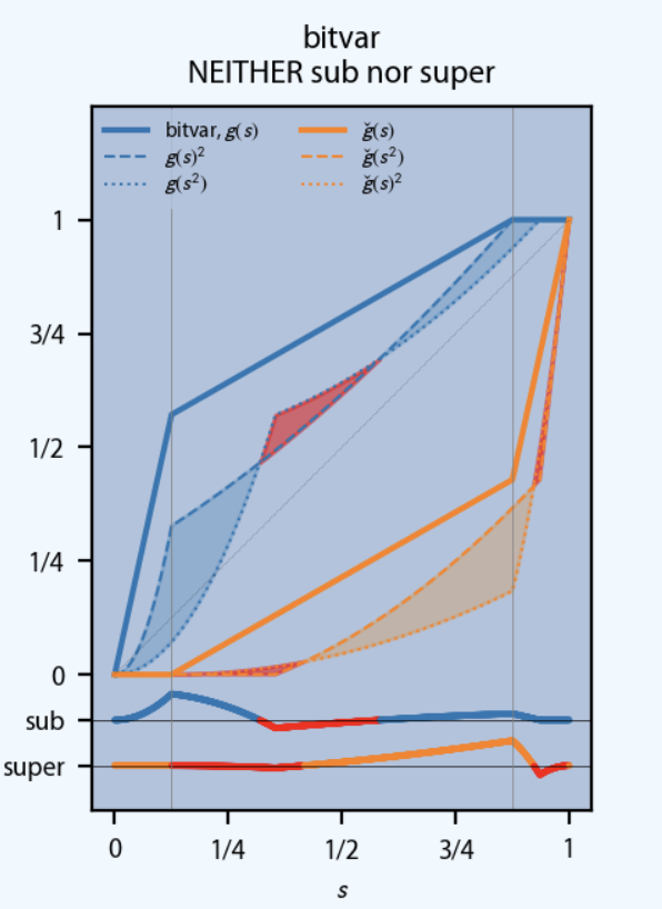
Figure 4.13: Sub- and super-multiplicative properties of a proper BiTVaR by varying $p_0$ and $p_1$ with $w=1/2$. The black and white lines plot example distortions, the alternating color is just for contrast.

Proof (Proof of correctness of (alg-040-exact-max-h?)). We prove that the algorithm returns the exact global maximum of $h$ over $[0,1]^2$.

Start by partitioning $[0,1]^2$ into kink-cells, with boundaries in the kink set $\{x_0,\dots,x_n\}$. Add

vertical lines at $s=x_i$,
horizontal lines at $t=x_j$,
hyperbolas $st=x_k$.

A kink-cell is a region where the segment indices of $s$, $t$, and $st$ are fixed: \[ s\in[x_i,x_{i+1}],\quad t\in[x_j,x_{j+1}],\quad st\in[x_k,x_{k+1}]. \] On such a cell, \[ g(s)=m_i s + b_i,\quad g(t)=m_j t + b_j,\quad g(st)=m_k(st)+b_k, \] so \[ \begin{aligned} h(s,t) &= (m_k st+b_k)-(m_i s+b_i)(m_j t+b_j)\\ &= (m_k-m_i m_j)\,st - m_i b_j\,s - m_j b_i\,t + (b_k-b_i b_j). \end{aligned} \] Thus on each kink-cell, $h$ is a bilinear function of $(s,t)$ of the form \[ h(s,t)=\alpha\,st+\beta\,s+\gamma\,t+\delta. \]

Bilinear functions have no strict 2D interior extrema on a rectangle. Fix $t$. On a kink-cell, $h(\cdot,t)$ is affine in $s$. Therefore, for each fixed $t$, the maximum over $s$ on the interval is attained at an endpoint. Equivalently, if $R=[u_0,u_1]\times[v_0,v_1]$ is a rectangle and $h$ is bilinear on $R$, then \[ \max_{(s,t)\in R} h(s,t) \] is attained on the boundary $\partial R$. Applying this to each kink-cell shows that any global maximizer of $h$ on $[0,1]^2$ lies on the union of kink-cell boundaries. Thus, it suffices to maximize over cell boundaries.

The boundary of a kink-cell consists of pieces of three types:

vertical segments $s=x_i$ with $t$ varying,
horizontal segments $t=x_j$ with $s$ varying,
hyperbola arcs $st=x_k$ with $(s,t)$ varying along the curve.

We show that the algorithm’s candidate set includes maxima on each boundary piece.

Along a vertical boundary $s=x_i$, the segment index of $s$ is fixed and $h$ reduces to a piecewise affine function of $t$: \[ t\mapsto h(x_i,t). \] Within any interval where $t$ and $x_i t$ remain in fixed segments, this function is affine, hence its maximum on that interval is at an endpoint. Endpoints of such intervals occur exactly when:

$t$ hits a kink: $t=x_j$, or
$x_i t$ hits a kink: $x_i t = x_k$, i.e. $t=x_k/x_i$.

These points are precisely included in:

Step A: $(x_i,x_j)$ kink-grid points,
Step B: $(x_i,x_k/x_i)$ hyperbola–kink-line intersections.

The same reasoning applies to horizontal boundaries $t=x_j$, with endpoints at

$s=x_i$ and
$s=x_k/x_j$,

again covered by Steps A and B.

Thus all maxima on vertical/horizontal boundary segments are attained at points in the candidate set.

Next, consider a hyperbola boundary $st=c$ where $c=x_k$ is a kink. Restrict $h$ to the curve by parameterizing $t=c/s$ and defining \[ f(s)=h\!\left(s,\frac{c}{s}\right)=g(c)-g(s)g(c/s), \qquad s\in[c,1]. \] On any sub-arc where $g(s)$ and $g(c/s)$ are affine: \[ g(s)=m_i s+b_i,\qquad g(c/s)=m_j\frac{c}{s}+b_j, \] we have \[ \begin{aligned} f(s) &=g(c)-(m_i s+b_i)\left(m_j\frac{c}{s}+b_j\right)\\ &=\text{const}-(m_i b_j)s-(b_i m_j)\frac{c}{s}. \end{aligned} \] Thus on that sub-arc, \[ f(s)=\text{const}-A s-\frac{B}{s}, \qquad A=m_i b_j,\quad B=b_i m_j c. \] If $A>0$ and $B>0$, then \[ f''(s)=-\frac{2B}{s^3}<0, \] so $f$ is strictly concave and has at most one stationary point, which is a maximizer. The stationary condition is \[ f'(s)=0 \quad\Longleftrightarrow\quad -A+\frac{B}{s^2}=0 \quad\Longleftrightarrow\quad s^2=\frac{B}{A}=\frac{m_j b_i c}{m_i b_j}. \] So the unique stationary point is \[ s_*=\sqrt{\frac{m_j b_i c}{m_i b_j}}, \qquad t_*=\frac{c}{s_*}. \] Therefore, the maximum of $f$ on that sub-arc is attained either:

at an endpoint of the sub-arc, or
at $(s_*,t_*)$ if it lies inside the sub-arc.

Endpoints of the sub-arc occur exactly when $s$ or $t=c/s$ hits a kink line, i.e. \[ s=x_i\quad \text{or}\quad t=x_j, \] which are the hyperbola–kink-line intersections added in Step B.

The stationary point, when feasible, is added in Step C. If $A=0$ or $B=0$, then $f$ becomes affine in either $s$ or $1/s$ on that sub-arc, so its maximum is still attained at endpoints, already handled by Step B. Hence, maxima of $h$ on all hyperbola boundary arcs $st=c$ are attained at points in the candidate set.

In conclusion, we have shown:

Any global maximizer of $h$ lies on kink-cell boundaries.
On every boundary piece (vertical, horizontal, hyperbola), the maximum is attained at a point in the candidate set constructed by Steps A, B, and C.

Therefore, evaluating $h$ on the candidate set and taking the maximum returns the exact global maximum over $[0,1]^2$ and this proves the algorithm’s correctness.

../

Acciaio, Beatrice. 2007. “Optimal risk sharing with non-monotone monetary functionals.” Finance and Stochastics 11 (2): 267–89. https://doi.org/10.1007/s00780-007-0036-6.

Acerbi, Carlo. 2002. “Spectral measures of risk: A coherent representation of subjective risk aversion.” Journal of Banking & Finance 26 (7): 1505–18. https://doi.org/10.1016/S0378-4266(02)00281-9.

Albrecher, Hansjörg, Karl Theodor Eisele, Mogens Steffensen, and Mario V. Wüthrich. 2022. “On the cost-of-capital rate under incomplete market valuation.” Journal of Risk and Insurance 89 (4): 1139–58. https://doi.org/10.1111/jori.12406.

Aliprantis, Charalambos D., and Kim C. Border. 2006. Infinite Dimensional Analysis: A Hitchhiker’s Guide. Third. Springer Verlag. https://doi.org/10.1007/3-540-29587-9.

Artzner, Philippe, Freddy Delbaen, Jean-Marc Eber, and David C. Heath. 1999. “Coherent measures of risk.” Mathematical Finance 9 (3): 203–28. http://onlinelibrary.wiley.com/doi/10.1111/1467-9965.00068/abstract.

Boonen, Tim J. 2017. “Risk redistribution games with dual utilities.” ASTIN Bulletin 47 (1): 303–29. https://doi.org/10.1017/asb.2016.34.

Borch, Karl. 1962. “Equilibrium in a Reinsurance Market.” Econometrica 30 (3): 424–44.

Carlier, G., and R. A. Dana. 2003. “Core of convex distortions of a probability.” Journal of Economic Theory 113 (2): 199–222. https://doi.org/10.1016/S0022-0531(03)00122-4.

Carlier, G., and R. A. Dana. 2008. “Two-persons efficient risk-sharing and equilibria for concave law-invariant utilities.” Economic Theory 36 (2): 189–223. https://doi.org/10.1007/s00199-007-0266-z.

Castagnoli, Erio, Fabio Maccheroni, and Massimo Marinacci. 2002. “Insurance premia consistent with the market.” Insurance: Mathematics and Economics 31 (2): 267–84. https://doi.org/10.1016/S0167-6687(02)00155-5.

Chateauneuf, A., R. Kast, and A. Lapied. 1996. “On Choquet pricing for financial markets with frictions.” Mathematical Finance 6 (3): 323–30. https://doi.org/10.1111/j.1467-9965.1996.tb00119.x.

Cherny, Alexander S., and Dmitri Orlov. 2011. “On two approaches to coherent risk contribution.” Mathematical Finance 21 (3): 557–71. https://doi.org/10.1111/j.1467-9965.2010.00441.x.

Choquet, Gustave. 1954. “Theory of capacities.” Ann Inst Fourier 5: 131–295. https://doi.org/10.5802/aif.53.

De Waegenaere, Anja. 2000. “Arbitrage and Viability in Insurance Markets.” GENEVA Papers on Risk and Insurance Theory 25 (1): 81–99. https://doi.org/10.1023/A:1008701608588.

De Waegenaere, Anja, Robert Kast, and Andre Lapied. 2003. “Choquet pricing and equilibrium.” Insurance: Mathematics and Economics 32: 359–70. https://doi.org/10.1016/S0167-6687(03)00116-1.

Delbaen, Freddy. 2000. “Coherent risk measures (Pisa Notes).” Pisa Notes 24 (4): 733–39. https://doi.org/10.1007/BF02809088.

Dellacherie, Claude. 1972. Capacités et processus stochastiques. Springer-Verlag.

Denuit, Michel M., and Jan Dhaene. 2012. “Convex order and comonotonic conditional mean risk sharing.” Insurance: Mathematics and Economics 51 (2): 265–70. https://doi.org/10.1016/j.insmatheco.2012.04.005.

Denuit, Michel M., Patricia Ortega-jimenez, and Christian Y. Robert. 2024. “Conditional Expectations Given The Sum Of Independent Random Variables With Regularly Varying Densities.” UCLouvain. https://dial.uclouvain.be/pr/boreal/object/boreal\%3A285506/datastream/PDF\_01/view.

Denuit, Michel M., Patricia Ortega-Jiménez, and Christian-Yann Robert. 2025. “Conditional expectations given the sum of independent random variables with regularly varying densities.” ASTIN Bulletin, ahead of print. https://doi.org/10.1017/asb.2025.11.

Dickson, David CM, Mary R. Hardy, and Howard R. Waters. 2015. Actuarial Mathematics for Life Contingent Risks. Vol. 1. Cambridge University Press. https://doi.org/10.1017/CBO9781107415324.004.

Efron, Bradley. 1965. “Increasing Properties of Polya Frequency Function.” The Annals of Mathematical Statistics, ahead of print. https://doi.org/10.1214/aoms/1177700288.

Filipović, Damir, and Gregor Svindland. 2008. “Optimal capital and risk allocations for law- and cash-invariant convex functions.” Finance and Stochastics 12 (3): 423–39. https://doi.org/10.1007/s00780-008-0069-5.

Föllmer, Hans, and Alexander Schied. 2016. Stochastic Finance: An Introduction in Discrete Time. Fourth. Walter de Gruyter. https://doi.org/10.1017/CBO9781107415324.004.

Grechuk, Bogdan. 2015. “The center of a convex set and capital allocation.” European Journal of Operational Research 243 (2): 628–36. https://doi.org/10.1016/j.ejor.2014.12.004.

Hewitt, Edwin. 1960. “Integration by Parts for Stieltjes Integrals.” The American Mathematical Monthly 67 (5): 419. https://doi.org/10.2307/2309287.

Jouini, E., W. Schachermayer, and N. Touzi. 2008. “Optimal risk sharing for law invariant monetary utility functions.” Mathematical Finance 18 (2): 269–92. https://doi.org/10.1111/j.1467-9965.2007.00332.x.

Kusuoka, Shigeo. 2001. “On law invariant coherent risk measures.” Advances in Mathematical Economics 3: 83–95. http://link.springer.com/chapter/10.1007/978-4-431-67891-5\_4.

Landsberger, Michael, and Isaac Meilijson. 1994. “Co-monotone allocations, Bickel-Lehmann dispersion and the Arrow-Pratt measure of risk aversion.” Annals of Operations Research 52 (2): 97–106. https://doi.org/10.1007/BF02033185.

Ludkovski, Michael, and Virginia R. Young. 2009. “Optimal risk sharing under distorted probabilities.” Mathematics and Financial Economics 2 (2): 87–105. https://doi.org/10.1007/s11579-009-0015-0.

Mahul, Olivier. 2003. “Efficient Risk Sharing within a Catastrophe Insurance Pool.” Paper Presented at the 2003 NBER Insurance Project Workshop, no. October.

Marinacci, Massimo, and Luigi Montrucchio. 2003. Introduction to the Mathematics of Ambiguity.

Marinacci, Massimo, and Luigi Montrucchio. 2004. “A characterization of the core of convex games through Gateaux derivatives.” Journal of Economic Theory 116 (2): 229–48. https://doi.org/10.1016/S0022-0531(03)00258-8.

Mildenhall, Stephen J., and John A. Major. 2022. Pricing Insurance Risk: Theory and Practice. John Wiley & Sons, Inc. https://doi.org/10.1002/9781119756538.

Rothschild, Michael, and Joseph E. Stiglitz. 1970. “Increasing risk: I. A definition.” Journal of Economic Theory 2 (3): 225–43. https://doi.org/10.1016/0022-0531(70)90038-4.

Ryff, John V. 1970. “Measure preserving transformations and rearrangements.” Journal of Mathematical Analysis and Applications 31 (2): 449–58. https://doi.org/10.1016/0022-247X(70)90038-7.

Saumard, Adrien, and Jon A. Wellner. 2014. “Log-concavity and strong log-concavity: a review.” Statistics Surveys 8: 45–114. https://doi.org/10.1214/14-SS107.

Schmeidler, David. 1986. “Integral representation without additivity.” Proceedings of the American Mathematical Society 97 (2): 255–55. https://doi.org/10.1090/S0002-9939-1986-0835875-8.

Simon, Barry. 2011. Convexity: an analytic viewpoint. Vol. 187. Cambridge University Press.

Stone, James M. 1973. “A Theory of Capacity and the Insurance of Catastrophe Risks (Part II).” The Journal of Risk and Insurance 40 (3): 339–55. https://doi.org/10.2307/252115.

Svindland, Gregor. 2014. “Dilatation monotonicity and convex order.” Mathematics and Financial Economics 8 (3): 241–47. https://doi.org/10.1007/s11579-013-0112-y.

Tsanakas, Andreas, and E. Desli. 2003. “Risk Measures and Theories of Choice.” British Actuarial Journal 9 (04): 959–91. https://doi.org/10.1017/S1357321700004414.

Venter, Gary G., John A. Major, and Rodney E. Kreps. 2006. “Marginal Decomposition of Risk Measures.” ASTIN Bulletin 36 (2): 375–413. https://doi.org/10.2143/AST.36.2.2017927.

Wang, Shaun S. 1996. “Premium Calculation by Transforming the Layer Premium Density.” ASTIN Bulletin 26 (01): 71–92. https://doi.org/10.2143/AST.26.1.563234.

Wang, Shaun S. 2000. “A class of distorion operators for pricing financial and insurance risks.” Journal of Risk and Insurance 67 (1): 15–36.

Yaari, Menahem E. 1987. “The Dual Theory of Choice under Risk.” The Econometric Society 55 (1): 95–115.

Distortion	Formula	Parameter
CCoC	\(\nu s+\delta\)	\(\iota=0.1500\)
PH	\(s^\alpha\)	\(\alpha=0.7205\)
Wang	\(\Phi(\Phi^{-1}(s)+\lambda)\)	\(\lambda=0.3427\)
Dual	\(1-(1-s)^m\)	\(m=1.5951\)
TVaR	\(1\wedge s/(1-p)\)	\(p=0.2713\)

Name	\(g(t)\)	\(g'(1-t)\) spectral function	\(\mu(dp)\) TVaR weight measure
CCoC	\((\delta + \nu t)\set{t>0}\)	\(\delta\set{t=1} + \nu\set{t<1}\)	\(\delta\set{p=1} + \nu\set{p=0}\)
PH	\(t^a\)	\(a(1-t)^{a-1}\)	\(a(1-a)(1-p)^{a-1} \, dt + a\set{p=0}\)
Wang	\(\Phi(\Phi^{-1}(t) + \lambda)\)	\(e^{\lambda \Phi^{-1}(t) - \lambda^2/2}\)	\(-(1-p)g''(1-p) \, dp\)
Dual	\(1 - (1-t)^b\)	\(b t^{b-1}\)	\(b(b-1)(1-p)t^{b-2} \, dp\)
TVaR	\(1\wedge \dfrac{t}{1-p}\)	\(\dfrac{1}{1-p} \set{t > p}\)	\(\delta_{p}\)

Property of \(g\)	Why Essential
\(g(0)=0\), \(g(1)=1\)	\(c=g\mathsf P\) is normalized.
Increasing	\(c\) is monotone
Convex	\(c\) submodular and hence \(\rho\) is subadditive

Column	Formula
A	\(x_i\), sorted in ascending in rows 2 to \(n+1\)
B	\(p_i\), check \(p_i\ge 0\) and sum to 1
C	\(F_i=\mathrm{SUM}(B2{:}B\set{n+1})\), cumulative probabilities
D	\(=1-Ci\), \(S_i=1-F_i\), exceedance probabilities
E	\(E1=0, Ei = D\set{i-1}\), shifts survival down and prepend 1, \(S_0=1, S_{i-1}\)
F	\(g p_i=g(E_i)-g(D_i)\), difference to obtain risk adjusted probs
G	contribution \(=A_i\times F_i\)
G total	\(g[X]=\mathrm{SUM}(G)\).

Distortion	Parameter	Parameter in \(p\)	Price

TVaR	\(p\)	\(p\)	\(\dfrac{1+p}{2}\)
Dual	\(b\)	\(\dfrac{1+p}{1-p}\)	\(\dfrac{b}{1+b}\)
Wang	\(\lambda\)	\(\sqrt2\Phi^{-1}\left(\dfrac{1+p}2\right)\)	\(\Phi\left(\dfrac\lambda{\sqrt2}\right)\)
PH	\(a\)	\(\dfrac{1-p}{1+p}\)	\(\dfrac1{1+a}\)
CCoC	\(\delta\)	\(p\)	\(\dfrac{1+\delta}2\)

Name	Low \(p_0\)	High \(p_1\)	\(s=0\)	\(s=1\)	SBM	SPM	Box Color
Mean	\(p_0=0\)	\(p_1=0\)	n/a\({}^{1}\)	n/a\({}^{1}\)	Yes\(^{\,2}\)	Yes\(^{\,2}\)	Black M
Max	\(p_0=1\)	\(p_1=1\)	n/a\({}^{10}\)	n/a\({}^{10}\)	Yes\(^{\,9}\)	Yes\(^{\,9}\)	Black X
TVaR	\(p_0>0\)	\(p_1=p_0<1\)	\(\check S\)	\(\check M\)	Yes\(^{\,8}\)	No\(^{\,4,7}\)	Green
CCoC	\(p_0=0\)	\(p_1=1\)	\(M\)	\(S\)	No\(^{\,3,5}\)	Yes\(^{\,6}\)	Black C
Mean-BiTVaR	\(p_0=0\)	\(p_1<1\)	\(\check S\)	\(S\)	No\(^{\,3}\)	No\(^{\,4}\)	Orange
Max-BiTVaR	\(p_0>0\)	\(p_1=1\)	\(M\)	\(\check M\)	No\(^{\,5}\)	No\(^{\,7}\)	Purple
BiTVaR\(_{b}\)	\(p_0>0\)	\(p_1<1\)	\(\check S\)	\(\check M\)	Yes\(^{\,11}\)	No\(^{\,4,7}\)	Grey
BiTVaR	\(p_0>0\)	\(p_1<1\)	\(\check S\)	\(\check M\)	No\(^{\,11}\)	No\(^{\,4,7}\)	Red

4.1 Single-Period Pricing

4.2 Bernoulli Risks and Their Pricing

4.3 Distortion Functions

4.3.1 Definition of a Distortion Function

4.3.2 Five Representative Distortion Functions

4.3.3 Concavity and Its Importance

4.3.4 The Dual of a Distortion

4.3.5 Transformations of \(g\) and Their Economic Meaning

4.3.6 TVaR as Extreme Points and the Kusuoka Correspondence

4.3.7 The Spectrum of a Distortion

4.4 Spectral Risk Measures

4.4.1 The Survival Function Expression for the Mean

4.4.2 The Layer-Cake Representation for Positive Random Variables

4.4.3 Capacities and the Choquet Integral

4.4.4 Six Representations of the Choquet Integrals

4.4.5 The Spectral Representation Theorem I

4.4.6 Calibrating Distortions to Market Pricing

4.4.7 The Spectral Representation Theorem II

4.5 The Natural Allocation

4.5.1 Preliminary Definition of the NA

4.5.2 The NA is a Marginal Cost

4.5.3 Properties of NA Prices

4.5.4 NA Prices, Underwriting, and Financing

4.5.5 Caveats

4.6 The Linear Natural Allocation

4.6.1 The Problem of Ties

4.6.2 Technical Result

4.7 Risk Sharing and \(g\)-Economies

4.7.1 The Market: Actors, Endowments, and Preferences

4.7.2 Jouini’s Risk Sharing Result

4.7.3 Feasibility

4.7.4 Solvency and Default

4.7.5 Asset Endowments and Binding Capacity

4.7.6 Inefficiency and the Role of Intermediation

4.7.7 Examples

4.7.8 Financial Sector

Chateauneuf et al. (1996) (135 citations) Choquet pricing for financial markets with frictions

De Waegenaere (2000) (3 citations) Arbitrage and Viability in Insurance Markets

Castagnoli et al. (2002) (56 citations) Insurance premia consistent with the market

De Waegenaere et al. (2003) (48 citations) Choquet pricing and equilibrium

4.7.9 Other Lit

Jouini et al. (2008) (245 citations) Optimal risk sharing for law invariant monetary utility functions

Filipović and Svindland (2008) (129 citations) Optimal capital and risk allocations for law- and cash-invariant convex functions

Carlier and Dana (2008) (61 citations) Two-persons efficient risk-sharing and equilibria for concave law-invariant utilities

Ludkovski and Young (2009) (50 citations) Optimal risk sharing under distorted probabilities

Boonen (2017) (3 citations) Risk redistribution games with dual utilities

4.8 The Switcheroo Trick and Understanding Diversification

4.8.1 The Switcheroo Trick: A Huge Simplification

4.8.2 \(\kappa\), diversifiable risk, and the small unit problem

4.8.3 Application with Limited Liability

4.8.4 Linear Natural Allocation Algorithm with Switcheroo

4.8.5 Examples of the Linear Natural Allocation

4.8.6 Why the Reduction Matters

4.9 Understanding Diversification Through the Switcheroo Trick

4.9.1 The Default Zone

4.9.2 Decomposing \(\kappa\): insurance and financing components

4.9.3 The Three Pricing Regimes

4.9.4 Examples

4.9.5 Jordan Decomposition of Finite Variation Functions

4.10 Advanced Properties of Distortions

4.10.1 Multiplicative Properties of Distortions

4.10.2 Conditions for SBM and SPM

4.10.3 BiTVaRs

4.10.4 Algorithm to determine \(\max h\) for a Weighted TVaR

Algorithm ExactMaxMultiplicativityExcess(g)

4.10.5 TriTVaRs

4.10.6 Elasticity

4.10.7 Properties of the Representative Distortions

4.10.8 Proofs

../

Algorithm `ExactMaxMultiplicativityExcess(g)`