Compiled: 2026-02-28 09:47:25.4555616003 Bullets and Discounting
posts/030-bullets.qmd

Pricing depends on ultimate loss volatility, payout pattern, emergence, and the accounting convention. A bullet policy fixes the payout pattern. We consider GAAP and IFRS accounting, and (eventually) a range of emergence and volatility assumptions.
TODO mention nice early discussion of Philbrick (1994): types of risk margin = certainty equivalent (IFRS 17), theory of ruin; probability intervals (APRA); relative measure of risk; interestingly not market value / cost to transfer (S2). Then discusses accounting. single-, three-period and steady-state models.
3.1 Bullet Payment Insurance Contracts
posts/030-files/bullets.qmd
This section describes bullet insurance contracts that settle with a single payment at a known time. We can learn a surprising amount from the accounting of these seemingly trivial examples. Bullets are useful because they separate emergence from payout: the ultimate value of a bullet can emerge over multiple period even though the loss is settled with one payment. The examples reveal that GAAP and IFRS differ in the speed of income recognition and the split between insurance and investment operations. To focus solely on discount, the examples in this section assume a fixed payment amount, made and known at a fixed time. The bullet contract is used extensively in later examples as a building block for units with multi-period payout patterns.
3.1.1 Deterministic Bullet Payment Assumptions
In a loan, a bullet payment is a single payment of the entire remaining balance of a loan or bond on its maturity date. That motivates the next definition.
Definition 3.1 A bullet is an insurance contract that settles with a single payment at a specified future time.
The bullet accounting examples assume:
- one-year contract term,
- loss paid at time \(T\),
- expected loss amount \(L\),
- premium \(P\) earned evenly over the policy term,
- premium is collected at \(t=0\), and
- the insurer earns \(r_a\) on invested assets.
These six assumptions apply to both GAAP and IFRS views. We need two further IFRS-specific assumptions:
- the market-based IFRS loss discount rate is \(r_I\) (see Section 2.3.10), and
- the entity-specific IFRS risk adjustment amount \(\mathrm{RA}\) and its release pattern.
The risk adjustment is quite subtle and is discussed further in ?nte-bullets-bullets-risk-adjustment.
Remark 3.1 (The Risk Adjustment: Balance Sheet versus Pricing Views). Under IFRS 17, the risk adjustment for non-financial risk (RA) represents the compensation an insurer requires for bearing the uncertainty of future cash flows. Conceptually, it is the excess of a risk-adjusted valuation over the mean: \[ \mathrm{RA}_t = \mathsf Q\left( \text{PV}_t[L] \right) - \text{PV}_t[\mathsf P L], \] where \(L\) is the stochastic loss payment stream, \(\text{PV}_t[\cdot]\) denotes present value at time \(t\) using the liability discount rate, and \(\mathsf Q\) is the risk-adjusted (pricing) probability.
Balance-sheet view
At each reporting date \(t\), the booked risk adjustment is a discounted liability balance that evolves by \[ \mathrm{RA}_{t} = (1 + r_I)\mathrm{RA}_{t-1} - R_{t},\quad t=2,\dots \tag{2.1} \] where
- \(r_I\) is the accretion rate consistent with the fulfilment cash flow discount rate, and
- \(R_t\) is the release of risk adjustment recognized in the income statement for period \(t\).
The total income-statement impact is the net of accretion and release: \[ \Delta \mathrm{RA}_t = \mathrm{RA}_t - \mathrm{RA}_{t-1} = r_I\mathrm{RA}_{t-1} - R_t . \] The accretion is charged against investment income as the insurance finance charge and the release is a negative insurance expense—hence generating income. IFRS prescribes that the release pattern \({\bar \pi_t}\) be based on how uncertainty is expected to reduce, typically proportional to incurred claims or other coverage units. Then the release, which occurs at the end of the period, is \[ R_t = \bar \pi_t\mathrm{RA}_{t-1}(1+r_I), \quad \bar \pi_t \ge 0. \tag{2.2} \] Thus IFRS starts from the booked balance and applies a risk adjustment pattern \(\bar \pi_t\) to determine recognized release.
The total balance sheet risk adjustment booked at \(t\) is then the discounted sum of these expected releases \[ \mathrm{RA}_t = \sum_{i \ge t+1} v_I^{i-t} R_i, \tag{2.3} \] by backward induction.
Pricing or earnings-pattern view
A pricing actuary instead thinks forwards: uncertainty resolves through time, generating expected nominal releases \(R_t\) with total \(R=\sum_{t\ge 2} R_t\). The implied nominal recognition pattern \(\rho_t = R_t / R\), \(t=2,\dots,T\) is often easier to calibrate directly to experience, e.g., proportional to expected loss emergence or volatility decline. By definition, \(\rho_t\ge 0\) and \(\sum_t \rho_t = 1\).
Relation to the CSM
The RA is a balance-sheet component that runs off with uncertainty; the Contractual Service Margin (CSM) is the residual profit deferral ensuring no gain at inception. In pricing terms, the CSM at issue can be viewed heuristically as the needed risk adjustment at $t=1 plus a service margin—the variable that reconciles the pricing equation to the given premium. The RA carries forward as a liability for incurred risk; the CSM is the off-balance component for unearned profit. Importantly, IFRS regards the risk adjustments as fixed independent of pricing and computes the service margin from premium. As a result, any premium inadequacy is recognized at inception in the insurance loss. It is subsequently earned back over time as the risk adjustment releases.
Formula Reconciliation
- Balance sheet or reserving view: \(\mathrm{RA}_t\) risk adjustment on balance sheet at \(t=1,2,\dots\)
- Income statement or pricing view: \(R_t\) amount of risk adjustment released at \(t=2,\dots\), \(R:=\sum_{t\ge 2} R_t\).
- \(\bar\pi_t\) is the risk adjustment pattern, giving \(R_t = \mathrm{RA}_{t-1}(1 + r_I) \bar\pi_t\) for \(t=2,\dots,T\), the proportion of the end of period risk adjustment released into income. \(\bar\pi_T=1\) to ensure all the risk adjustment is ultimately released.
- \(\rho_t = R_t / R\), \(t=2,\dots\) is the corresponding risk adjustment recognition pattern.
All releases and balance sheet items are end-of-period.
The pricing release pattern \(\rho_t\) can then be converted into a risk adjustment pattern via \[ R_t = \rho_t \mathrm{RA} \\ \bar\pi_t = R_t / ((1 + r_I)\mathrm{RA}_{t-1}). \]
All \(\bar\pi_i \ge 0\), but they do not sum to 1 because they are a proportion of the outstanding recognized at each point. They can be converted into a normalized cumulative release pattern \(\pi_i\) summing to 1 via \[ \begin{aligned} \pi_2 &= \bar\pi_2 \\ \pi_i &= \frac{\bar\pi_i}{(1-\bar\pi_2)\cdots(1 - \bar\pi_{i-1})}, & i =3,\dots, T. \end{aligned} \]
A pricing actuary would include an amount \(R_1\), the amount released at \(t=1\), and work with a pattern relative to \(R':=R_1 + R\). However, \(R_1\) is not considered by the reserving actuary—it has been released before they begin work. To work with \(R_1\), re-scale the patterns by computing \(\rho'_t = R_t/R'\) and \(\rho_i = \rho'_i / (1-\rho'_1)\).
All of these formulae are easy to program in a single-sweep manner using Python’s accumulate and reduce functions.
not clear where this should go
Table 3.1 lays out the assumptions for a five-year bullet payment. The risk adjustment is earned equally over the 4 years after the policy term.
The pro formas assume the maximum allowed dividend is paid, subject to cash and retained income constraints, Section 2.3.5. That means dividends can only be paid when cumulative retained earnings are positive—you can’t pay dividends out of capital—and the cash must both be available to pay the dividend—you can’t borrow to pay. In this case, since the contract is profitable and the premium is collected at inception, the dividend equals the operating result in each period.
| Variable | Value | Comments |
|---|---|---|
| 2025-01-01 | Policy effective date | |
| \(T\) | 5 | Duration of loss payment |
| \(L\) | 1000 | Expected losses |
| \(P\) | 980 | EPV loss plus risk adjustment |
| \(\text{RA}_1\) | 100 | IFRS risk adjustment booked at \(t=1\) |
| \(r_a\) | 0.05 | Investment yield on invested assets |
| \(r_I\) | 0.035 | IFRS interest rate for discounting losses |
| Pattern | Equal | Risk adjustment earned equally |
Under GAAP there is an underwriting loss recognized in the first period that is gradually offset by a stream of investment income, see Table 3.2 (a)-(c). Here, and in the other tables in this section, zero values are shown as dashes to avoid distracting entries.
Under IFRS there is a small insurance service profit in the first year since losses are discounted and the discount exceeds the risk adjustment. Notice the two offsetting effects: deferring the risk adjustment slows income recognition and discounting speeds it up. The net effect depends on specific assumptions. These effects are show in Table 3.2 (d)-(f).
| Period Ending | Starting Cash | Premium Collected | Investment Income | Loss Paid | Dividends Paid | Net Cash Flow | Capital Paid-In | Ending Cash |
|---|---|---|---|---|---|---|---|---|
| 2025/12/31 | - | 980 | 49 | - | 29 | 1,000 | - | 1,000 |
| 2026/12/31 | 1,000 | - | 50 | - | 50 | - | - | 1,000 |
| 2027/12/31 | 1,000 | - | 50 | - | 50 | - | - | 1,000 |
| 2028/12/31 | 1,000 | - | 50 | - | 50 | - | - | 1,000 |
| 2029/12/31 | 1,000 | - | 50 | 1,000 | 50 | -1,000 | - | - |
| Period Ending | Cash | Loss Reserve | UPR | Capital Paid-In | Retained Earnings | Equity |
|---|---|---|---|---|---|---|
| 2025/12/31 | 1,000 | 1,000 | - | - | - | - |
| 2026/12/31 | 1,000 | 1,000 | - | - | - | - |
| 2027/12/31 | 1,000 | 1,000 | - | - | - | - |
| 2028/12/31 | 1,000 | 1,000 | - | - | - | - |
| 2029/12/31 | - | - | - | - | - | - |
| Period Ending | Earned Premium | Loss Incurred | Underwriting Result | Net Investment Income | Operating Result | Dividends | Change in Equity |
|---|---|---|---|---|---|---|---|
| 2025/12/31 | 980 | 1,000 | -20 | 49 | 29 | 29 | - |
| 2026/12/31 | - | - | - | 50 | 50 | 50 | - |
| 2027/12/31 | - | - | - | 50 | 50 | 50 | - |
| 2028/12/31 | - | - | - | 50 | 50 | 50 | - |
| 2029/12/31 | - | - | - | 50 | 50 | 50 | - |
| Period Ending | Starting Cash | Premium Collected | Investment Income | Loss Paid | Dividends Paid | Net Cash Flow | Capital Paid-In | Ending Cash |
|---|---|---|---|---|---|---|---|---|
| 2025/12/31 | - | 980 | 49 | - | 57.6 | 971 | - | 971 |
| 2026/12/31 | 971 | - | 48.6 | - | 40.4 | 8.13 | - | 980 |
| 2027/12/31 | 980 | - | 49 | - | 41.5 | 7.5 | - | 987 |
| 2028/12/31 | 987 | - | 49.4 | - | 42.5 | 6.83 | - | 994 |
| 2029/12/31 | 994 | - | 49.7 | 1,000 | 43.6 | -994 | - | - |
| Period Ending | Cash | Best Estimate Liability | Risk Adjustment | Liability for Remaining Coverage | Liability for Incurred Claims | Capital Paid-In | Retained Earnings | Equity |
|---|---|---|---|---|---|---|---|---|
| 2025/12/31 | 971 | 871 | 100 | - | 971 | - | - | - |
| 2026/12/31 | 980 | 902 | 77.6 | - | 980 | - | - | - |
| 2027/12/31 | 987 | 934 | 53.6 | - | 987 | - | - | - |
| 2028/12/31 | 994 | 966 | 27.7 | - | 994 | - | - | - |
| 2029/12/31 | - | - | - | - | - | - | - | - |
| Period Ending | Insurance Service Revenue | Insurance Service Expense | Insurance Service Result | Net Investment Income | Insurance Finance Expense | Investment Result | Operating Result | Dividends | Change in Equity |
|---|---|---|---|---|---|---|---|---|---|
| 2025/12/31 | 980 | 971 | 8.56 | 49 | - | 49 | 57.6 | 57.6 | - |
| 2026/12/31 | - | -25.9 | 25.9 | 48.6 | 34 | 14.6 | 40.4 | 40.4 | - |
| 2027/12/31 | - | -26.8 | 26.8 | 49 | 34.3 | 14.7 | 41.5 | 41.5 | - |
| 2028/12/31 | - | -27.7 | 27.7 | 49.4 | 34.5 | 14.8 | 42.5 | 42.5 | - |
| 2029/12/31 | - | -28.7 | 28.7 | 49.7 | 34.8 | 14.9 | 43.6 | 43.6 | - |
The GAAP accounting is straightforward. The IFRS accounting may be unfamiliar, so we provide more details. The statement of financial position (balance sheet), Table 3.2 (e) shows that the RA is deferred at the end of period 1. The RA is an input, along with premium, loss, etc. The best estimate liability (BEL) is equals the expected present value of losses at \(r_I\), and is combined with the RA to determine the liability for incurred claims (LIC), i.e., reserves. In subsequent years, the discount is amortized, which increases the BEL. However, since all is going according to plan there is no loss incurred running through the insurance service result. Instead, discount amortization is charged against the investment result, effectively crediting the investment income at rate \(r_I\) to the policyholder, see (f). Treating amortization in this way neatly divides investment income into an amount due to the policyholder and a net amount for the insurer, which is philosophically aligned with US statutory ratemaking procedures.
The risk adjustment is also amortized as uncertainty about ultimate losses resolves. By assumption, in this example it amortizes equally over \(T\) periods, but its exact pattern is a very important topic in the monograph and is discussed in REF. In order for premium (insurance service revenue) to be fixed at the end of the policy term, the release of RA is booked as a negative insurance expense. This also aligns with its being part of the insurance liability: it is like a release of reserves. The negative expense generates a positive insurance service result for each period. Only the accrual items depend on accounting, not the cash flows, except that the accruals determine dividends which feed into cash flows. This is an important example of the real-world impact of accounting standards.
Table 3.3 and Figure 3.1 display the profit source over time, showing how the operating result is split into underwriting and investment components by accounting type. GAAP (left) shows the only underwriting income, a loss, is reported in the first period, despite losses emerging over multiple years, and that more than 100% of the operating result is attributed to investment income! In contrast, IFRS (right) shows that some underwriting income is earned in each year as the risk emerges. The preponderance of the operating result is now associated with underwriting activities. The investment results reflect compensation for generating the spread \(r_a>r_I\) in returns. The smaller the spread (less skill in investing) the greater the proportion of income attributed to underwriting. The IFRS presentation better matches the business reality:
- The insurer’s business is insurance: the accounting should correctly reflect the importance of underwriting in generating economics.
- All of the funds invested are loaned by the policyholder—no investor surplus is shown.
- There is very little special investment skill deployed, evinced by the small spread \(r_a>r_I\).
- The RA makes conservatism in the reserves is explicit and disclosed.
| GAAP | IFRS | |||||||
|---|---|---|---|---|---|---|---|---|
| Period Ending | Underwriting Result | Net Investment Income | Operating Result | Dividends | Insurance Service Result | Investment Result | Operating Result | Dividends |
| 2025/12/31 | -20 | 49 | 29 | 29 | 8.56 | 49 | 57.6 | 57.6 |
| 2026/12/31 | - | 50 | 50 | 50 | 25.9 | 14.6 | 40.4 | 40.4 |
| 2027/12/31 | - | 50 | 50 | 50 | 26.8 | 14.7 | 41.5 | 41.5 |
| 2028/12/31 | - | 50 | 50 | 50 | 27.7 | 14.8 | 42.5 | 42.5 |
| 2029/12/31 | - | 50 | 50 | 50 | 28.7 | 14.9 | 43.6 | 43.6 |
| Total | -20 | 249 | 229 | 229 | 118 | 108 | 226 | 226 |
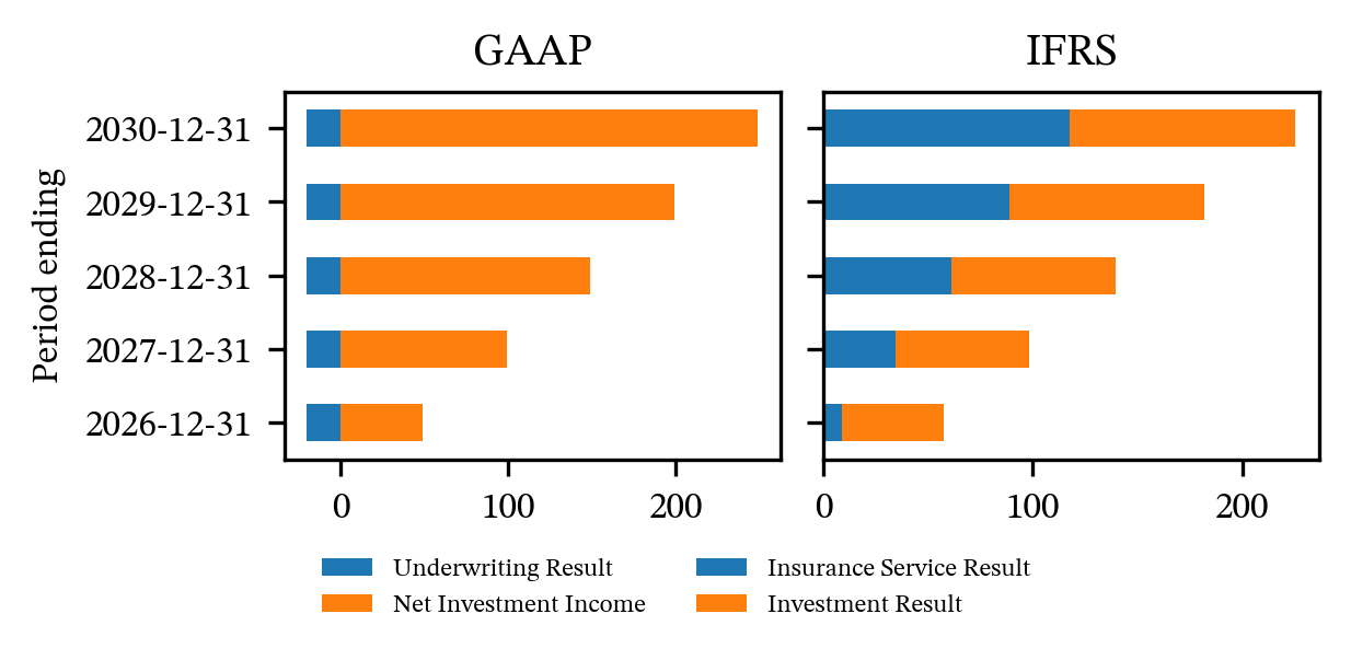
Table 3.4 shows the impact of removing dividends. Accounting determines dividends, paying dividends reduces cash, reduces investment income, and income and cash in subsequent periods. In Table 3.3 total operating results differ by accounting, whereas here they are the same: a real-world effect. Generally, in the absence of dividends, GAAP and IFRS cash flow statements are identical, as is the ending equity which can be computed by moving the \(t=0\) present value of all cash flows forward to time \(T\) using the investment yield \(r_y\) and is equal to \[ (P - Lv_a^{T}) (1+r_a)^T = RA (1+r_a)^T. \]
| GAAP | IFRS | |||||||
|---|---|---|---|---|---|---|---|---|
| Period Ending | Underwriting Result | Net Investment Income | Operating Result | Dividends | Insurance Service Result | Investment Result | Operating Result | Dividends |
| 2025/12/31 | -20 | 49 | 29 | - | 8.56 | 49 | 57.6 | - |
| 2026/12/31 | - | 51.5 | 51.5 | - | 25.9 | 17.4 | 43.3 | - |
| 2027/12/31 | - | 54 | 54 | - | 26.8 | 19.7 | 46.5 | - |
| 2028/12/31 | - | 56.7 | 56.7 | - | 27.7 | 22.2 | 49.9 | - |
| 2029/12/31 | - | 59.6 | 59.6 | - | 28.7 | 24.8 | 53.5 | - |
| Total | -20 | 271 | 251 | - | 118 | 133 | 251 | - |
3.1.2 A Loss Making Contract
Table 3.5 shows the effect of lowering premium so the contract makes a loss at initial recognition. Initial recognition under IFRS includes the risk adjustment expense. Technically, IFRS requires an insurance liability be set up for loss making contracts to recognize the loss immediately, but we do not consider it because it is typically not relevant for prospective pricing. Notwithstanding that point, the insurance loss is recognized at \(t=1\) in both conventions. This lowers the starting equity below zero and acts to restrict dividends until the loss has been offset by earned RA and investment income.
| GAAP | IFRS | |||||||
|---|---|---|---|---|---|---|---|---|
| Period Ending | Underwriting Result | Net Investment Income | Operating Result | Dividends | Insurance Service Result | Investment Result | Operating Result | Dividends |
| 2025/12/31 | -145 | 42.8 | -102 | - | -116 | 42.8 | -73.7 | - |
| 2026/12/31 | - | 44.9 | 44.9 | - | 25.9 | 10.9 | 36.8 | - |
| 2027/12/31 | - | 47.1 | 47.1 | - | 26.8 | 12.8 | 39.6 | 2.7 |
| 2028/12/31 | - | 49.5 | 49.5 | 39.3 | 27.7 | 14.8 | 42.5 | 42.5 |
| 2029/12/31 | - | 50 | 50 | 50 | 28.7 | 14.9 | 43.6 | 43.6 |
| Total | -145 | 234 | 89.3 | 89.3 | -7.38 | 96.2 | 88.8 | 88.8 |
3.1.3 GAAP is a Special Case Of IFRS
Table 3.6 shows that GAAP is a special case of IFRS, where the IFRS discount rate \(r_I\) is \(0\%\) and the deferred risk adjustment is zero. As a result, any margin in premium is earned in first period. This equivalence emphasizes that IFRS provides two levers to adjust income recognition compared to GAAP: the IFRS discount rate and the risk adjustment and its recognition pattern. The former is calibrated using market observables and depends on the liquidity characteristics of the policy. The latter is entity-specific. Together, they better align income recognition with the provision of risk bearing services.
| GAAP | IFRS | |||||||
|---|---|---|---|---|---|---|---|---|
| Period Ending | Underwriting Result | Net Investment Income | Operating Result | Dividends | Insurance Service Result | Investment Result | Operating Result | Dividends |
| 2025/12/31 | -20 | 49 | 29 | 29 | -20 | 49 | 29 | 29 |
| 2026/12/31 | - | 50 | 50 | 50 | - | 50 | 50 | 50 |
| 2027/12/31 | - | 50 | 50 | 50 | - | 50 | 50 | 50 |
| 2028/12/31 | - | 50 | 50 | 50 | - | 50 | 50 | 50 |
| 2029/12/31 | - | 50 | 50 | 50 | - | 50 | 50 | 50 |
| Total | -20 | 249 | 229 | 229 | -20 | 249 | 229 | 229 |
In general, varying the IFRS interest rate and risk adjustment alters the timing of income recognition and its split between insurance and investment operations. For example, by setting \(r_I=r_a\) and the risk adjustment to exactly offset amortization of interest in each period would convert all investment income into insurance income.
3.1.4 The Profit Signature
The profit signature describes when profits emerge: it is defined as the expected temporal pattern of profit emergence from a portfolio of insurance contracts, measured on a consistent accounting basis. It is commonly used in life insurance (Dickson et al. 2015). Profit emergence reflects the release of risk adjustment, interest accretion, and any experience variances recognized in the period. In an inter-temporal analysis, the attractiveness of a policy depends on how the profit signature aligns with the capital requirements of the policy. The profit signature can be presented on a cash, operating, or dividend basis, Table 3.7.
| GAAP | IFRS | |||||
|---|---|---|---|---|---|---|
| Period Ending | Cash Flow | Operating Result | Dividends | Cash Flow | Operating Result | Dividends |
| 2025/12/31 | 1,000 | 29 | 29 | 971 | 57.6 | 57.6 |
| 2026/12/31 | - | 50 | 50 | 8.13 | 40.4 | 40.4 |
| 2027/12/31 | - | 50 | 50 | 7.5 | 41.5 | 41.5 |
| 2028/12/31 | - | 50 | 50 | 6.83 | 42.5 | 42.5 |
| 2029/12/31 | -1,000 | 50 | 50 | -994 | 43.6 | 43.6 |
| Total | - | 229 | 229 | - | 226 | 226 |
3.1.5 Evaluating Premium
Investors must assess the adequacy of the profit signature stream compared to the risk of the policy. The textbook solution suggested by the profit signature is to look at the NPV of the dividend flows. However, as we discussed in Section 2.1.2, textbook NPV solutions make assumptions that do not hold for insurance. Ignoring those objections, Table 3.8 shows the present value of cash flows at different discount rates (cost of capital) across all scenarios. These present values should be compared to the potential capital calls. Table 3.9 compares valuations for each of the four scenarios considered so far using different costs of capital.
COMMENT ON SPEED and DIFFS BETWEEN ACCOUNTINGS.
| GAAP | IFRS | |||||
|---|---|---|---|---|---|---|
| Cost of Capital | Cash Flow | Operating Result | Dividends | Cash Flow | Operating Result | Dividends |
| 0.00% | - | 229 | 229 | - | 226 | 226 |
| 5.00% | 177 | 206 | 206 | 174 | 206 | 206 |
| 10.00% | 317 | 187 | 187 | 311 | 190 | 190 |
| 15.00% | 428 | 172 | 172 | 420 | 177 | 177 |
| 20.00% | 518 | 158 | 158 | 508 | 166 | 166 |
| 25.00% | 590 | 147 | 147 | 579 | 156 | 156 |
| GAAP | IFRS | ||||||
|---|---|---|---|---|---|---|---|
| Scenario | Cost of Capital | Cash Flow | Operating Result | Dividends | Cash Flow | Operating Result | Dividends |
| Base | 0.00% | 0 | 229 | 229 | 0 | 226 | 226 |
| 5.00% | 177 | 206 | 206 | 174 | 206 | 206 | |
| 10.00% | 317 | 187 | 187 | 311 | 190 | 190 | |
| 15.00% | 428 | 172 | 172 | 420 | 177 | 177 | |
| 20.00% | 518 | 158 | 158 | 508 | 166 | 166 | |
| 25.00% | 590 | 147 | 147 | 579 | 156 | 156 | |
| Loss making | 0.00% | 0 | 89 | 89 | 0 | 89 | 89 |
| 5.00% | 169 | 67 | 75 | 169 | 70 | 75 | |
| 10.00% | 302 | 49 | 64 | 302 | 54 | 64 | |
| 15.00% | 407 | 34 | 54 | 407 | 41 | 55 | |
| 20.00% | 492 | 21 | 47 | 491 | 30 | 48 | |
| 25.00% | 559 | 10 | 41 | 558 | 21 | 41 | |
| No dividends | 0.00% | 251 | 251 | 0 | 251 | 251 | 0 |
| 5.00% | 402 | 225 | 0 | 402 | 228 | 0 | |
| 10.00% | 521 | 204 | 0 | 521 | 209 | 0 | |
| 15.00% | 614 | 186 | 0 | 614 | 194 | 0 | |
| 20.00% | 689 | 171 | 0 | 689 | 181 | 0 | |
| 25.00% | 749 | 158 | 0 | 749 | 169 | 0 | |
| GAAP Special Case | 0.00% | 0 | 229 | 229 | 0 | 229 | 229 |
| 5.00% | 177 | 206 | 206 | 177 | 206 | 206 | |
| 10.00% | 317 | 187 | 187 | 317 | 187 | 187 | |
| 15.00% | 428 | 172 | 172 | 428 | 172 | 172 | |
| 20.00% | 518 | 158 | 158 | 518 | 158 | 158 | |
| 25.00% | 590 | 147 | 147 | 590 | 147 | 147 | |
Table 3.10 shows the implied pricing discount rates \(r_p\), computed so that premium equals \(v_p^{-T}\mathsf PX\). A lower rate corresponds to a more adequate premium because it requires less discount.
| Scenario | Pricing discount rate |
|---|---|
| Base | 0.405% |
| Loss making | 3.183% |
| No dividends | 0.405% |
| GAAP Special Case | 0.405% |
3.2 Building General Units from Bullets
3.2.1 Units with Multi-year Payout Patterns
This section shows how to build a unit with a multi-year payout pattern by combining bullets. Table 3.11 shows the bullets needed to achieve a payout pattern of 10%, 30%, 30%, 20%, 10% over five years. The remaining assumptions are the same as Table 3.1, and, for simplicity, premium and risk adjustment are handled pro rata.
| 2025 | Total | ||||||
|---|---|---|---|---|---|---|---|
| Category | Item | 1 | 2 | 3 | 4 | 5 | |
| Contract Details | Name | (2025, 1) | (2025, 2) | (2025, 3) | (2025, 4) | (2025, 5) | Total |
| Policy duration | 1 | 2 | 3 | 4 | 5 | 1.5 | |
| Dates | Policy effective date | 2025/01/01 | 2025/01/01 | 2025/01/01 | 2025/01/01 | 2025/01/01 | 2025/01/01 |
| Policy end date | 2025/12/31 | 2025/12/31 | 2025/12/31 | 2025/12/31 | 2025/12/31 | 2025/12/31 | |
| Payout_date | 2025/12/31 | 2026/12/31 | 2027/12/31 | 2028/12/31 | 2029/12/31 | 2025/12/31 | |
| Core Economics | Premium | 98 | 294 | 294 | 196 | 98 | 980 |
| Expected Loss | 100 | 300 | 300 | 200 | 100 | 1000 | |
| Dividend Payout | 1 | 1 | 1 | 1 | 1 | 1 | |
| Rates | IFRS Yield | 0.035 | 0.035 | 0.035 | 0.035 | 0.035 | 0.035 |
| Asset Yield | 0.05 | 0.05 | 0.05 | 0.05 | 0.05 | 0.05 | |
| Priced Yield | 0.0204 | 0.0102 | 0.0068 | 0.0051 | 0.004 | nan | |
| Risk Adjustment | Risk Adjustment | 0 | 33.3333 | 33.3333 | 22.2222 | 11.1111 | 100 |
| IFRS Results | PV Loss (IFRS Rate) | 96.6184 | 280.0532 | 270.5828 | 174.2884 | 84.1973 | 218.1301 |
| PV Cash Flow (IFRS Rate) | 1.3816 | 13.9468 | 23.4172 | 21.7116 | 13.8027 | 74.2599 | |
| CSM | 1.3816 | -19.3865 | -9.9161 | -0.5107 | 2.6916 | -25.7401 | |
| Economic Value | PV Cash Flow (Asset Yield) | 2.7619 | 21.8912 | 34.8487 | 31.4595 | 19.6474 | 110.6087 |
| FV Cash Flow (Asset Yield) | 2.9 | 24.135 | 40.3418 | 38.2392 | 25.0756 | 130.6916 | |
Table 3.12 shows the resulting accounting pro formas as the reserves run off. These statements can be decomposed by payout lag adding the argument details=True.
| Period Ending | Starting Cash | Premium Collected | Investment Income | Loss Paid | Dividends Paid | Net Cash Flow | Capital Paid-In | Ending Cash |
|---|---|---|---|---|---|---|---|---|
| 2025/12/31 | - | 980 | 49 | 100 | 29 | 900 | - | 900 |
| 2026/12/31 | 900 | - | 45 | 300 | 45 | -300 | - | 600 |
| 2027/12/31 | 600 | - | 30 | 300 | 30 | -300 | - | 300 |
| 2028/12/31 | 300 | - | 15 | 200 | 15 | -200 | - | 100 |
| 2029/12/31 | 100 | - | 5 | 100 | 5 | -100 | - | - |
| Period Ending | Cash | Loss Reserve | UPR | Capital Paid-In | Retained Earnings | Equity |
|---|---|---|---|---|---|---|
| 2025/12/31 | 900 | 900 | - | - | - | - |
| 2026/12/31 | 600 | 600 | - | - | - | - |
| 2027/12/31 | 300 | 300 | - | - | - | - |
| 2028/12/31 | 100 | 100 | - | - | - | - |
| 2029/12/31 | - | - | - | - | - | - |
| Period Ending | Earned Premium | Loss Incurred | Underwriting Result | Net Investment Income | Operating Result | Dividends | Change in Equity |
|---|---|---|---|---|---|---|---|
| 2025/12/31 | 980 | 1,000 | -20 | 49 | 29 | 29 | - |
| 2026/12/31 | - | - | - | 45 | 45 | 45 | - |
| 2027/12/31 | - | - | - | 30 | 30 | 30 | - |
| 2028/12/31 | - | - | - | 15 | 15 | 15 | - |
| 2029/12/31 | - | - | - | 5 | 5 | 5 | - |
| Period Ending | Starting Cash | Premium Collected | Investment Income | Loss Paid | Dividends Paid | Net Cash Flow | Capital Paid-In | Ending Cash |
|---|---|---|---|---|---|---|---|---|
| 2025/12/31 | - | 980 | 49 | 100 | 10.7 | 918 | - | 918 |
| 2026/12/31 | 918 | - | 45.9 | 300 | 56.2 | -310 | - | 608 |
| 2027/12/31 | 608 | - | 30.4 | 300 | 37.9 | -307 | - | 300 |
| 2028/12/31 | 300 | - | 15 | 200 | 15.8 | -201 | - | 99.7 |
| 2029/12/31 | 99.7 | - | 4.98 | 100 | 4.68 | -99.7 | - | - |
| Period Ending | Cash | Best Estimate Liability | Risk Adjustment | Liability for Remaining Coverage | Liability for Incurred Claims | Capital Paid-In | Retained Earnings | Equity |
|---|---|---|---|---|---|---|---|---|
| 2025/12/31 | 918 | 837 | 100 | - | 937 | - | -19.2 | -19.2 |
| 2026/12/31 | 608 | 567 | 41.2 | - | 608 | - | - | - |
| 2027/12/31 | 300 | 287 | 13.9 | - | 300 | - | - | - |
| 2028/12/31 | 99.7 | 96.6 | 3.08 | - | 99.7 | - | - | - |
| 2029/12/31 | - | - | - | - | - | - | - | - |
| Period Ending | Insurance Service Revenue | Insurance Service Expense | Insurance Service Result | Net Investment Income | Insurance Finance Expense | Investment Result | Operating Result | Dividends | Change in Equity |
|---|---|---|---|---|---|---|---|---|---|
| 2025/12/31 | 980 | 1,040 | -57.4 | 49 | - | 49 | -8.44 | 10.7 | -19.2 |
| 2026/12/31 | - | -62.3 | 62.3 | 45.9 | 32.8 | 13.1 | 75.4 | 56.2 | 19.2 |
| 2027/12/31 | - | -28.8 | 28.8 | 30.4 | 21.3 | 9.12 | 37.9 | 37.9 | - |
| 2028/12/31 | - | -11.3 | 11.3 | 15 | 10.5 | 4.51 | 15.8 | 15.8 | - |
| 2029/12/31 | - | -3.19 | 3.19 | 4.98 | 3.49 | 1.5 | 4.68 | 4.68 | - |
As with a bullet, we can add a full reserve history, Table 3.13. In this case, the exhibits show the underlying detail for the current calendar year. Panels (f) and (g) are worth studying; they show how IFRS explicitly displays released earnings as uncertainty unwinds, and amortization of interest over time.
| effective | payout | Starting Cash | Premium Collected | Investment Income | Loss Paid | Dividends Paid | Net Cash Flow | Capital Paid-In | Ending Cash |
|---|---|---|---|---|---|---|---|---|---|
| 2021 | 1 | - | - | - | - | - | - | - | - |
| 2 | - | - | - | - | - | - | - | - | |
| 3 | - | - | - | - | - | - | - | - | |
| 4 | - | - | - | - | - | - | - | - | |
| 5 | 74.9 | - | 3.74 | 74.9 | 3.74 | -74.9 | - | - | |
| 2022 | 1 | - | - | - | - | - | - | - | - |
| 2 | - | - | - | - | - | - | - | - | |
| 3 | - | - | - | - | - | - | - | - | |
| 4 | 161 | - | 8.05 | 161 | 8.05 | -161 | - | - | |
| 5 | 80.5 | - | 4.02 | - | 4.02 | - | - | 80.5 | |
| 2023 | 1 | - | - | - | - | - | - | - | - |
| 2 | - | - | - | - | - | - | - | - | |
| 3 | 260 | - | 13 | 260 | 13 | -260 | - | - | |
| 4 | 173 | - | 8.65 | - | 8.65 | - | - | 173 | |
| 5 | 86.5 | - | 4.33 | - | 4.33 | - | - | 86.5 | |
| 2024 | 1 | - | - | - | - | - | - | - | - |
| 2 | 279 | - | 14 | 279 | 14 | -279 | - | - | |
| 3 | 279 | - | 14 | - | 14 | - | - | 279 | |
| 4 | 186 | - | 9.3 | - | 9.3 | - | - | 186 | |
| 5 | 93 | - | 4.65 | - | 4.65 | - | - | 93 | |
| 2025 | 1 | - | 98 | 4.9 | 100 | 2.9 | - | - | - |
| 2 | - | 294 | 14.7 | - | 8.7 | 300 | - | 300 | |
| 3 | - | 294 | 14.7 | - | 8.7 | 300 | - | 300 | |
| 4 | - | 196 | 9.8 | - | 5.8 | 200 | - | 200 | |
| 5 | - | 98 | 4.9 | - | 2.9 | 100 | - | 100 | |
| Total | 1,670 | 980 | 133 | 875 | 113 | 125 | - | 1,800 |
| effective | payout | Cash | Loss Reserve | UPR | Capital Paid-In | Retained Earnings | Equity |
|---|---|---|---|---|---|---|---|
| 2021 | 1 | - | - | - | - | - | - |
| 2 | - | - | - | - | - | - | |
| 3 | - | - | - | - | - | - | |
| 4 | - | - | - | - | - | - | |
| 5 | - | - | - | - | - | - | |
| 2022 | 1 | - | - | - | - | - | - |
| 2 | - | - | - | - | - | - | |
| 3 | - | - | - | - | - | - | |
| 4 | - | - | - | - | - | - | |
| 5 | 80.5 | 80.5 | - | - | - | - | |
| 2023 | 1 | - | - | - | - | - | - |
| 2 | - | - | - | - | - | - | |
| 3 | - | - | - | - | - | - | |
| 4 | 173 | 173 | - | - | - | - | |
| 5 | 86.5 | 86.5 | - | - | - | - | |
| 2024 | 1 | - | - | - | - | - | - |
| 2 | - | - | - | - | - | - | |
| 3 | 279 | 279 | - | - | - | - | |
| 4 | 186 | 186 | - | - | - | - | |
| 5 | 93 | 93 | - | - | - | - | |
| 2025 | 1 | - | - | - | - | - | - |
| 2 | 300 | 300 | - | - | - | - | |
| 3 | 300 | 300 | - | - | - | - | |
| 4 | 200 | 200 | - | - | - | - | |
| 5 | 100 | 100 | - | - | - | - | |
| Total | 1,800 | 1,800 | - | - | - | - |
| effective | payout | Earned Premium | Loss Incurred | Underwriting Result | Net Investment Income | Operating Result | Dividends | Change in Equity |
|---|---|---|---|---|---|---|---|---|
| 2021 | 1 | - | - | - | - | - | - | - |
| 2 | - | - | - | - | - | - | - | |
| 3 | - | - | - | - | - | - | - | |
| 4 | - | - | - | - | - | - | - | |
| 5 | - | - | - | 3.74 | 3.74 | 3.74 | - | |
| 2022 | 1 | - | - | - | - | - | - | - |
| 2 | - | - | - | - | - | - | - | |
| 3 | - | - | - | - | - | - | - | |
| 4 | - | - | - | 8.05 | 8.05 | 8.05 | - | |
| 5 | - | - | - | 4.02 | 4.02 | 4.02 | - | |
| 2023 | 1 | - | - | - | - | - | - | - |
| 2 | - | - | - | - | - | - | - | |
| 3 | - | - | - | 13 | 13 | 13 | - | |
| 4 | - | - | - | 8.65 | 8.65 | 8.65 | - | |
| 5 | - | - | - | 4.33 | 4.33 | 4.33 | - | |
| 2024 | 1 | - | - | - | - | - | - | - |
| 2 | - | - | - | 14 | 14 | 14 | - | |
| 3 | - | - | - | 14 | 14 | 14 | - | |
| 4 | - | - | - | 9.3 | 9.3 | 9.3 | - | |
| 5 | - | - | - | 4.65 | 4.65 | 4.65 | - | |
| 2025 | 1 | 98 | 100 | -2 | 4.9 | 2.9 | 2.9 | - |
| 2 | 294 | 300 | -6 | 14.7 | 8.7 | 8.7 | - | |
| 3 | 294 | 300 | -6 | 14.7 | 8.7 | 8.7 | - | |
| 4 | 196 | 200 | -4 | 9.8 | 5.8 | 5.8 | - | |
| 5 | 98 | 100 | -2 | 4.9 | 2.9 | 2.9 | - | |
| Total | 980 | 1,000 | -20 | 133 | 113 | 113 | - |
| effective | payout | TW Start Cash | TW Premium | TW Loss Paid | TW Capital | Average Cash Balance |
|---|---|---|---|---|---|---|
| 2021 | 1 | - | - | - | - | - |
| 2 | - | - | - | - | - | |
| 3 | - | - | - | - | - | |
| 4 | - | - | - | - | - | |
| 5 | 74.9 | - | - | - | 74.9 | |
| 2022 | 1 | - | - | - | - | - |
| 2 | - | - | - | - | - | |
| 3 | - | - | - | - | - | |
| 4 | 161 | - | - | - | 161 | |
| 5 | 80.5 | - | - | - | 80.5 | |
| 2023 | 1 | - | - | - | - | - |
| 2 | - | - | - | - | - | |
| 3 | 260 | - | - | - | 260 | |
| 4 | 173 | - | - | - | 173 | |
| 5 | 86.5 | - | - | - | 86.5 | |
| 2024 | 1 | - | - | - | - | - |
| 2 | 279 | - | - | - | 279 | |
| 3 | 279 | - | - | - | 279 | |
| 4 | 186 | - | - | - | 186 | |
| 5 | 93 | - | - | - | 93 | |
| 2025 | 1 | - | 98 | - | - | 98 |
| 2 | - | 294 | - | - | 294 | |
| 3 | - | 294 | - | - | 294 | |
| 4 | - | 196 | - | - | 196 | |
| 5 | - | 98 | - | - | 98 | |
| Total | 1,670 | 980 | - | - | 2,650 |
| effective | payout | Starting Cash | Premium Collected | Investment Income | Loss Paid | Dividends Paid | Net Cash Flow | Capital Paid-In | Ending Cash |
|---|---|---|---|---|---|---|---|---|---|
| 2021 | 1 | - | - | - | - | - | - | - | - |
| 2 | - | - | - | - | - | - | - | - | |
| 3 | - | - | - | - | - | - | - | - | |
| 4 | - | - | - | - | - | - | - | - | |
| 5 | 74.7 | - | 3.73 | 74.9 | 3.51 | -74.7 | - | - | |
| 2022 | 1 | - | - | - | - | - | - | - | - |
| 2 | - | - | - | - | - | - | - | - | |
| 3 | - | - | - | - | - | - | - | - | |
| 4 | 162 | - | 8.1 | 161 | 9.04 | -162 | - | - | |
| 5 | 79.9 | - | 4 | - | 3.68 | 0.319 | - | 80.3 | |
| 2023 | 1 | - | - | - | - | - | - | - | - |
| 2 | - | - | - | - | - | - | - | - | |
| 3 | 266 | - | 13.3 | 260 | 19.4 | -266 | - | - | |
| 4 | 175 | - | 8.74 | - | 9.49 | -0.747 | - | 174 | |
| 5 | 85.5 | - | 4.28 | - | 3.86 | 0.418 | - | 85.9 | |
| 2024 | 1 | - | - | - | - | - | - | - | - |
| 2 | 287 | - | 14.4 | 279 | 22.5 | -287 | - | - | |
| 3 | 287 | - | 14.4 | - | 15.8 | -1.48 | - | 286 | |
| 4 | 188 | - | 9.42 | - | 9.96 | -0.535 | - | 188 | |
| 5 | 91.4 | - | 4.57 | - | 4.05 | 0.525 | - | 91.9 | |
| 2025 | 1 | - | 98 | 4.9 | 100 | 2.9 | - | - | - |
| 2 | - | 294 | 14.7 | - | - | 309 | - | 309 | |
| 3 | - | 294 | 14.7 | - | - | 309 | - | 309 | |
| 4 | - | 196 | 9.8 | - | 3.19 | 203 | - | 203 | |
| 5 | - | 98 | 4.9 | - | 4.64 | 98.3 | - | 98.3 | |
| Total | 1,700 | 980 | 134 | 875 | 112 | 127 | - | 1,820 |
| effective | payout | Cash | Best Estimate Liability | Risk Adjustment | Liability for Remaining Coverage | Liability for Incurred Claims | Capital Paid-In | Retained Earnings | Equity |
|---|---|---|---|---|---|---|---|---|---|
| 2021 | 1 | - | - | - | - | - | - | - | - |
| 2 | - | - | - | - | - | - | - | - | |
| 3 | - | - | - | - | - | - | - | - | |
| 4 | - | - | - | - | - | - | - | - | |
| 5 | - | - | - | - | - | - | - | - | |
| 2022 | 1 | - | - | - | - | - | - | - | - |
| 2 | - | - | - | - | - | - | - | - | |
| 3 | - | - | - | - | - | - | - | - | |
| 4 | - | - | - | - | - | - | - | - | |
| 5 | 80.3 | 77.8 | 2.48 | - | 80.3 | - | - | - | |
| 2023 | 1 | - | - | - | - | - | - | - | - |
| 2 | - | - | - | - | - | - | - | - | |
| 3 | - | - | - | - | - | - | - | - | |
| 4 | 174 | 167 | 6.87 | - | 174 | - | - | - | |
| 5 | 85.9 | 80.8 | 5.15 | - | 85.9 | - | - | - | |
| 2024 | 1 | - | - | - | - | - | - | - | - |
| 2 | - | - | - | - | - | - | - | - | |
| 3 | 286 | 270 | 16 | - | 286 | - | - | - | |
| 4 | 188 | 174 | 14.3 | - | 188 | - | - | - | |
| 5 | 91.9 | 83.9 | 8.02 | - | 91.9 | - | - | - | |
| 2025 | 1 | - | - | - | - | - | - | - | - |
| 2 | 309 | 290 | 33.3 | - | 323 | - | -14.5 | -14.5 | |
| 3 | 309 | 280 | 33.3 | - | 313 | - | -4.69 | -4.69 | |
| 4 | 203 | 180 | 22.2 | - | 203 | - | - | - | |
| 5 | 98.3 | 87.1 | 11.1 | - | 98.3 | - | - | - | |
| Total | 1,820 | 1,690 | 153 | - | 1,840 | - | -19.2 | -19.2 |
| effective | payout | Insurance Service Revenue | Insurance Service Expense | Insurance Service Result | Net Investment Income | Insurance Finance Expense | Investment Result | Operating Result | Dividends | Change in Equity |
|---|---|---|---|---|---|---|---|---|---|---|
| 2021 | 1 | - | - | - | - | - | - | - | - | - |
| 2 | - | - | - | - | - | - | - | - | - | |
| 3 | - | - | - | - | - | - | - | - | - | |
| 4 | - | - | - | - | - | - | - | - | - | |
| 5 | - | -2.39 | 2.39 | 3.73 | 2.61 | 1.12 | 3.51 | 3.51 | - | |
| 2022 | 1 | - | - | - | - | - | - | - | - | - |
| 2 | - | - | - | - | - | - | - | - | - | |
| 3 | - | - | - | - | - | - | - | - | - | |
| 4 | - | -6.61 | 6.61 | 8.1 | 5.67 | 2.43 | 9.04 | 9.04 | - | |
| 5 | - | -2.48 | 2.48 | 4 | 2.8 | 1.2 | 3.68 | 3.68 | - | |
| 2023 | 1 | - | - | - | - | - | - | - | - | - |
| 2 | - | - | - | - | - | - | - | - | - | |
| 3 | - | -15.4 | 15.4 | 13.3 | 9.3 | 3.99 | 19.4 | 19.4 | - | |
| 4 | - | -6.87 | 6.87 | 8.74 | 6.12 | 2.62 | 9.49 | 9.49 | - | |
| 5 | - | -2.57 | 2.57 | 4.28 | 2.99 | 1.28 | 3.86 | 3.86 | - | |
| 2024 | 1 | - | - | - | - | - | - | - | - | - |
| 2 | - | -32.1 | 32.1 | 14.4 | 10.5 | 3.84 | 35.9 | 22.5 | 13.5 | |
| 3 | - | -16 | 16 | 14.4 | 10.2 | 4.15 | 20.2 | 15.8 | 4.36 | |
| 4 | - | -7.13 | 7.13 | 9.42 | 6.6 | 2.83 | 9.96 | 9.96 | - | |
| 5 | - | -2.67 | 2.67 | 4.57 | 3.2 | 1.37 | 4.05 | 4.05 | - | |
| 2025 | 1 | 98 | 100 | -2 | 4.9 | - | 4.9 | 2.9 | 2.9 | - |
| 2 | 294 | 323 | -29.2 | 14.7 | - | 14.7 | -14.5 | - | -14.5 | |
| 3 | 294 | 313 | -19.4 | 14.7 | - | 14.7 | -4.69 | - | -4.69 | |
| 4 | 196 | 203 | -6.61 | 9.8 | - | 9.8 | 3.19 | 3.19 | - | |
| 5 | 98 | 98.3 | -0.255 | 4.9 | - | 4.9 | 4.64 | 4.64 | - | |
| Total | 980 | 943 | 36.9 | 134 | 60 | 73.8 | 111 | 112 | -1.34 |
| effective | payout | TW Start Cash | TW Premium | TW Loss Paid | TW Capital | Average Cash Balance |
|---|---|---|---|---|---|---|
| 2021 | 1 | - | - | - | - | - |
| 2 | - | - | - | - | - | |
| 3 | - | - | - | - | - | |
| 4 | - | - | - | - | - | |
| 5 | 74.7 | - | - | - | 74.7 | |
| 2022 | 1 | - | - | - | - | - |
| 2 | - | - | - | - | - | |
| 3 | - | - | - | - | - | |
| 4 | 162 | - | - | - | 162 | |
| 5 | 79.9 | - | - | - | 79.9 | |
| 2023 | 1 | - | - | - | - | - |
| 2 | - | - | - | - | - | |
| 3 | 266 | - | - | - | 266 | |
| 4 | 175 | - | - | - | 175 | |
| 5 | 85.5 | - | - | - | 85.5 | |
| 2024 | 1 | - | - | - | - | - |
| 2 | 287 | - | - | - | 287 | |
| 3 | 287 | - | - | - | 287 | |
| 4 | 188 | - | - | - | 188 | |
| 5 | 91.4 | - | - | - | 91.4 | |
| 2025 | 1 | - | 98 | - | - | 98 |
| 2 | - | 294 | - | - | 294 | |
| 3 | - | 294 | - | - | 294 | |
| 4 | - | 196 | - | - | 196 | |
| 5 | - | 98 | - | - | 98 | |
| Total | 1,700 | 980 | - | - | 2,680 |
Table 3.14 shows the profit source and Table 3.15 adds the underlying details. The profit signature is also available with the same splits.
| GAAP | IFRS | |||||||
|---|---|---|---|---|---|---|---|---|
| Period Ending | Underwriting Result | Net Investment Income | Operating Result | Dividends | Insurance Service Result | Investment Result | Operating Result | Dividends |
| 2021/12/31 | -15 | 36.7 | 21.7 | 21.7 | -43 | 36.7 | -6.32 | 8.04 |
| 2022/12/31 | -16.1 | 73.1 | 57 | 57 | 0.406 | 49.3 | 49.7 | 50.7 |
| 2023/12/31 | -17.3 | 101 | 83.8 | 83.8 | 22 | 59.8 | 81.8 | 82.9 |
| 2024/12/31 | -18.6 | 120 | 101 | 101 | 32.1 | 67.6 | 99.7 | 101 |
| 2025/12/31 | -20 | 133 | 113 | 113 | 36.9 | 73.8 | 111 | 112 |
| 2026/12/31 | - | 89.9 | 89.9 | 89.9 | 101 | 26.7 | 128 | 109 |
| 2027/12/31 | - | 48.3 | 48.3 | 48.3 | 42 | 14.6 | 56.6 | 56.6 |
| 2028/12/31 | - | 19.7 | 19.7 | 19.7 | 14.3 | 5.9 | 20.2 | 20.2 |
| 2029/12/31 | - | 5 | 5 | 5 | 3.19 | 1.5 | 4.68 | 4.68 |
| Total | -87 | 626 | 539 | 539 | 209 | 336 | 545 | 545 |
| GAAP | IFRS | |||||||||
|---|---|---|---|---|---|---|---|---|---|---|
| Period Ending | Effective Year | Payout Lag | Underwriting Result | Net Investment Income | Operating Result | Dividends | Insurance Service Result | Investment Result | Operating Result | Dividends |
| 2021/12/31 | 2021 | 1 | -1.5 | 3.67 | 2.17 | 2.17 | -1.5 | 3.67 | 2.17 | 2.17 |
| 2 | -4.49 | 11 | 6.51 | 6.51 | -21.9 | 11 | -10.8 | - | ||
| 3 | -4.49 | 11 | 6.51 | 6.51 | -14.5 | 11 | -3.51 | - | ||
| 4 | -3 | 7.34 | 4.34 | 4.34 | -4.95 | 7.34 | 2.39 | 2.39 | ||
| 5 | -1.5 | 3.67 | 2.17 | 2.17 | -0.191 | 3.67 | 3.48 | 3.48 | ||
| 2022/12/31 | 2021 | 1 | - | - | - | - | - | - | - | - |
| 2 | - | 11.2 | 11.2 | 11.2 | 25.8 | 3.09 | 28.9 | 18.1 | ||
| 3 | - | 11.2 | 11.2 | 11.2 | 12.9 | 3.34 | 16.3 | 12.8 | ||
| 4 | - | 7.49 | 7.49 | 7.49 | 5.74 | 2.28 | 8.02 | 8.02 | ||
| 5 | - | 3.74 | 3.74 | 3.74 | 2.15 | 1.1 | 3.26 | 3.26 | ||
| 2022 | 1 | -1.61 | 3.94 | 2.33 | 2.33 | -1.61 | 3.94 | 2.33 | 2.33 | |
| 2 | -4.83 | 11.8 | 7 | 7 | -23.5 | 11.8 | -11.7 | - | ||
| 3 | -4.83 | 11.8 | 7 | 7 | -15.6 | 11.8 | -3.77 | - | ||
| 4 | -3.22 | 7.89 | 4.67 | 4.67 | -5.32 | 7.89 | 2.57 | 2.57 | ||
| 5 | -1.61 | 3.94 | 2.33 | 2.33 | -0.206 | 3.94 | 3.74 | 3.74 | ||
| 2023/12/31 | 2021 | 1 | - | - | - | - | - | - | - | - |
| 2 | - | - | - | - | - | - | - | - | ||
| 3 | - | 11.2 | 11.2 | 11.2 | 13.4 | 3.45 | 16.8 | 16.8 | ||
| 4 | - | 7.49 | 7.49 | 7.49 | 5.94 | 2.27 | 8.21 | 8.21 | ||
| 5 | - | 3.74 | 3.74 | 3.74 | 2.23 | 1.11 | 3.34 | 3.34 | ||
| 2022 | 1 | - | - | - | - | - | - | - | - | |
| 2 | - | 12.1 | 12.1 | 12.1 | 27.8 | 3.32 | 31.1 | 19.4 | ||
| 3 | - | 12.1 | 12.1 | 12.1 | 13.9 | 3.6 | 17.5 | 13.7 | ||
| 4 | - | 8.05 | 8.05 | 8.05 | 6.17 | 2.45 | 8.62 | 8.62 | ||
| 5 | - | 4.02 | 4.02 | 4.02 | 2.31 | 1.19 | 3.5 | 3.5 | ||
| 2023 | 1 | -1.73 | 4.24 | 2.51 | 2.51 | -1.73 | 4.24 | 2.51 | 2.51 | |
| 2 | -5.19 | 12.7 | 7.53 | 7.53 | -25.3 | 12.7 | -12.5 | - | ||
| 3 | -5.19 | 12.7 | 7.53 | 7.53 | -16.8 | 12.7 | -4.06 | - | ||
| 4 | -3.46 | 8.48 | 5.02 | 5.02 | -5.72 | 8.48 | 2.76 | 2.76 | ||
| 5 | -1.73 | 4.24 | 2.51 | 2.51 | -0.221 | 4.24 | 4.02 | 4.02 | ||
| 2024/12/31 | 2021 | 1 | - | - | - | - | - | - | - | - |
| 2 | - | - | - | - | - | - | - | - | ||
| 3 | - | - | - | - | - | - | - | - | ||
| 4 | - | 7.49 | 7.49 | 7.49 | 6.15 | 2.26 | 8.41 | 8.41 | ||
| 5 | - | 3.74 | 3.74 | 3.74 | 2.31 | 1.12 | 3.42 | 3.42 | ||
| 2022 | 1 | - | - | - | - | - | - | - | - | |
| 2 | - | - | - | - | - | - | - | - | ||
| 3 | - | 12.1 | 12.1 | 12.1 | 14.4 | 3.71 | 18.1 | 18.1 | ||
| 4 | - | 8.05 | 8.05 | 8.05 | 6.39 | 2.44 | 8.83 | 8.83 | ||
| 5 | - | 4.02 | 4.02 | 4.02 | 2.4 | 1.19 | 3.59 | 3.59 | ||
| 2023 | 1 | - | - | - | - | - | - | - | - | |
| 2 | - | 13 | 13 | 13 | 29.9 | 3.57 | 33.4 | 20.9 | ||
| 3 | - | 13 | 13 | 13 | 14.9 | 3.86 | 18.8 | 14.7 | ||
| 4 | - | 8.65 | 8.65 | 8.65 | 6.63 | 2.63 | 9.26 | 9.26 | ||
| 5 | - | 4.33 | 4.33 | 4.33 | 2.49 | 1.28 | 3.76 | 3.76 | ||
| 2024 | 1 | -1.86 | 4.56 | 2.7 | 2.7 | -1.86 | 4.56 | 2.7 | 2.7 | |
| 2 | -5.58 | 13.7 | 8.09 | 8.09 | -27.2 | 13.7 | -13.5 | - | ||
| 3 | -5.58 | 13.7 | 8.09 | 8.09 | -18 | 13.7 | -4.36 | - | ||
| 4 | -3.72 | 9.12 | 5.4 | 5.4 | -6.15 | 9.12 | 2.97 | 2.97 | ||
| 5 | -1.86 | 4.56 | 2.7 | 2.7 | -0.238 | 4.56 | 4.32 | 4.32 | ||
| 2025/12/31 | 2021 | 1 | - | - | - | - | - | - | - | - |
| 2 | - | - | - | - | - | - | - | - | ||
| 3 | - | - | - | - | - | - | - | - | ||
| 4 | - | - | - | - | - | - | - | - | ||
| 5 | - | 3.74 | 3.74 | 3.74 | 2.39 | 1.12 | 3.51 | 3.51 | ||
| 2022 | 1 | - | - | - | - | - | - | - | - | |
| 2 | - | - | - | - | - | - | - | - | ||
| 3 | - | - | - | - | - | - | - | - | ||
| 4 | - | 8.05 | 8.05 | 8.05 | 6.61 | 2.43 | 9.04 | 9.04 | ||
| 5 | - | 4.02 | 4.02 | 4.02 | 2.48 | 1.2 | 3.68 | 3.68 | ||
| 2023 | 1 | - | - | - | - | - | - | - | - | |
| 2 | - | - | - | - | - | - | - | - | ||
| 3 | - | 13 | 13 | 13 | 15.4 | 3.99 | 19.4 | 19.4 | ||
| 4 | - | 8.65 | 8.65 | 8.65 | 6.87 | 2.62 | 9.49 | 9.49 | ||
| 5 | - | 4.33 | 4.33 | 4.33 | 2.57 | 1.28 | 3.86 | 3.86 | ||
| 2024 | 1 | - | - | - | - | - | - | - | - | |
| 2 | - | 14 | 14 | 14 | 32.1 | 3.84 | 35.9 | 22.5 | ||
| 3 | - | 14 | 14 | 14 | 16 | 4.15 | 20.2 | 15.8 | ||
| 4 | - | 9.3 | 9.3 | 9.3 | 7.13 | 2.83 | 9.96 | 9.96 | ||
| 5 | - | 4.65 | 4.65 | 4.65 | 2.67 | 1.37 | 4.05 | 4.05 | ||
| 2025 | 1 | -2 | 4.9 | 2.9 | 2.9 | -2 | 4.9 | 2.9 | 2.9 | |
| 2 | -6 | 14.7 | 8.7 | 8.7 | -29.2 | 14.7 | -14.5 | - | ||
| 3 | -6 | 14.7 | 8.7 | 8.7 | -19.4 | 14.7 | -4.69 | - | ||
| 4 | -4 | 9.8 | 5.8 | 5.8 | -6.61 | 9.8 | 3.19 | 3.19 | ||
| 5 | -2 | 4.9 | 2.9 | 2.9 | -0.255 | 4.9 | 4.64 | 4.64 | ||
| 2026/12/31 | 2021 | 1 | - | - | - | - | - | - | - | - |
| 2 | - | - | - | - | - | - | - | - | ||
| 3 | - | - | - | - | - | - | - | - | ||
| 4 | - | - | - | - | - | - | - | - | ||
| 5 | - | - | - | - | - | - | - | - | ||
| 2022 | 1 | - | - | - | - | - | - | - | - | |
| 2 | - | - | - | - | - | - | - | - | ||
| 3 | - | - | - | - | - | - | - | - | ||
| 4 | - | - | - | - | - | - | - | - | ||
| 5 | - | 4.02 | 4.02 | 4.02 | 2.57 | 1.2 | 3.77 | 3.77 | ||
| 2023 | 1 | - | - | - | - | - | - | - | - | |
| 2 | - | - | - | - | - | - | - | - | ||
| 3 | - | - | - | - | - | - | - | - | ||
| 4 | - | 8.65 | 8.65 | 8.65 | 7.11 | 2.61 | 9.72 | 9.72 | ||
| 5 | - | 4.33 | 4.33 | 4.33 | 2.67 | 1.29 | 3.95 | 3.95 | ||
| 2024 | 1 | - | - | - | - | - | - | - | - | |
| 2 | - | - | - | - | - | - | - | - | ||
| 3 | - | 14 | 14 | 14 | 16.6 | 4.29 | 20.9 | 20.9 | ||
| 4 | - | 9.3 | 9.3 | 9.3 | 7.38 | 2.82 | 10.2 | 10.2 | ||
| 5 | - | 4.65 | 4.65 | 4.65 | 2.77 | 1.38 | 4.15 | 4.15 | ||
| 2025 | 1 | - | - | - | - | - | - | - | - | |
| 2 | - | 15 | 15 | 15 | 34.5 | 4.12 | 38.6 | 24.1 | ||
| 3 | - | 15 | 15 | 15 | 17.2 | 4.47 | 21.7 | 17 | ||
| 4 | - | 10 | 10 | 10 | 7.67 | 3.04 | 10.7 | 10.7 | ||
| 5 | - | 5 | 5 | 5 | 2.88 | 1.47 | 4.35 | 4.35 | ||
| 2027/12/31 | 2021 | 1 | - | - | - | - | - | - | - | - |
| 2 | - | - | - | - | - | - | - | - | ||
| 3 | - | - | - | - | - | - | - | - | ||
| 4 | - | - | - | - | - | - | - | - | ||
| 5 | - | - | - | - | - | - | - | - | ||
| 2022 | 1 | - | - | - | - | - | - | - | - | |
| 2 | - | - | - | - | - | - | - | - | ||
| 3 | - | - | - | - | - | - | - | - | ||
| 4 | - | - | - | - | - | - | - | - | ||
| 5 | - | - | - | - | - | - | - | - | ||
| 2023 | 1 | - | - | - | - | - | - | - | - | |
| 2 | - | - | - | - | - | - | - | - | ||
| 3 | - | - | - | - | - | - | - | - | ||
| 4 | - | - | - | - | - | - | - | - | ||
| 5 | - | 4.33 | 4.33 | 4.33 | 2.76 | 1.29 | 4.05 | 4.05 | ||
| 2024 | 1 | - | - | - | - | - | - | - | - | |
| 2 | - | - | - | - | - | - | - | - | ||
| 3 | - | - | - | - | - | - | - | - | ||
| 4 | - | 9.3 | 9.3 | 9.3 | 7.64 | 2.81 | 10.4 | 10.4 | ||
| 5 | - | 4.65 | 4.65 | 4.65 | 2.86 | 1.39 | 4.25 | 4.25 | ||
| 2025 | 1 | - | - | - | - | - | - | - | - | |
| 2 | - | - | - | - | - | - | - | - | ||
| 3 | - | 15 | 15 | 15 | 17.9 | 4.61 | 22.5 | 22.5 | ||
| 4 | - | 10 | 10 | 10 | 7.93 | 3.03 | 11 | 11 | ||
| 5 | - | 5 | 5 | 5 | 2.98 | 1.48 | 4.46 | 4.46 | ||
| 2028/12/31 | 2021 | 1 | - | - | - | - | - | - | - | - |
| 2 | - | - | - | - | - | - | - | - | ||
| 3 | - | - | - | - | - | - | - | - | ||
| 4 | - | - | - | - | - | - | - | - | ||
| 5 | - | - | - | - | - | - | - | - | ||
| 2022 | 1 | - | - | - | - | - | - | - | - | |
| 2 | - | - | - | - | - | - | - | - | ||
| 3 | - | - | - | - | - | - | - | - | ||
| 4 | - | - | - | - | - | - | - | - | ||
| 5 | - | - | - | - | - | - | - | - | ||
| 2023 | 1 | - | - | - | - | - | - | - | - | |
| 2 | - | - | - | - | - | - | - | - | ||
| 3 | - | - | - | - | - | - | - | - | ||
| 4 | - | - | - | - | - | - | - | - | ||
| 5 | - | - | - | - | - | - | - | - | ||
| 2024 | 1 | - | - | - | - | - | - | - | - | |
| 2 | - | - | - | - | - | - | - | - | ||
| 3 | - | - | - | - | - | - | - | - | ||
| 4 | - | - | - | - | - | - | - | - | ||
| 5 | - | 4.65 | 4.65 | 4.65 | 2.97 | 1.39 | 4.36 | 4.36 | ||
| 2025 | 1 | - | - | - | - | - | - | - | - | |
| 2 | - | - | - | - | - | - | - | - | ||
| 3 | - | - | - | - | - | - | - | - | ||
| 4 | - | 10 | 10 | 10 | 8.21 | 3.02 | 11.2 | 11.2 | ||
| 5 | - | 5 | 5 | 5 | 3.08 | 1.49 | 4.57 | 4.57 | ||
| 2029/12/31 | 2021 | 1 | - | - | - | - | - | - | - | - |
| 2 | - | - | - | - | - | - | - | - | ||
| 3 | - | - | - | - | - | - | - | - | ||
| 4 | - | - | - | - | - | - | - | - | ||
| 5 | - | - | - | - | - | - | - | - | ||
| 2022 | 1 | - | - | - | - | - | - | - | - | |
| 2 | - | - | - | - | - | - | - | - | ||
| 3 | - | - | - | - | - | - | - | - | ||
| 4 | - | - | - | - | - | - | - | - | ||
| 5 | - | - | - | - | - | - | - | - | ||
| 2023 | 1 | - | - | - | - | - | - | - | - | |
| 2 | - | - | - | - | - | - | - | - | ||
| 3 | - | - | - | - | - | - | - | - | ||
| 4 | - | - | - | - | - | - | - | - | ||
| 5 | - | - | - | - | - | - | - | - | ||
| 2024 | 1 | - | - | - | - | - | - | - | - | |
| 2 | - | - | - | - | - | - | - | - | ||
| 3 | - | - | - | - | - | - | - | - | ||
| 4 | - | - | - | - | - | - | - | - | ||
| 5 | - | - | - | - | - | - | - | - | ||
| 2025 | 1 | - | - | - | - | - | - | - | - | |
| 2 | - | - | - | - | - | - | - | - | ||
| 3 | - | - | - | - | - | - | - | - | ||
| 4 | - | - | - | - | - | - | - | - | ||
| 5 | - | 5 | 5 | 5 | 3.19 | 1.5 | 4.68 | 4.68 | ||
| Total | Total | Total | -87 | 626 | 539 | 539 | 209 | 336 | 545 | 545 |
3.3 Steady State Bullets
This section combines single bullets into a steadily growing portfolio, with prior year reserves rolling forward, and analyzes the calendar year financials. Then, Section 3.4 and Section 3.5 determine pricing to achieve overall profit margins under GAAP and IFRS. The objective is divide and conquer: start by solving this simple problem and then build up to realistic cases.
3.3.1 Growing Steady State Accounting Statements
Retain the assumptions from ?sec-bullets-bullet-payment-contracts shown in Table 3.1 and recapped in Table 3.16. To look at steady state exhibits we need to add four historical years with outstanding reserves. Assume that premium grows at 7.5% annually. Table 3.17 shows the relevant historical years. Table 3.18 shows the GAAP and IFRS financials, and illustrates the build-up and run-off of the 2025 position.
| Category | Item | Value |
|---|---|---|
| Contract Details | Name | (2025, 5) |
| Policy duration | 5 | |
| Dates | Policy effective date | 2025/01/01 |
| Policy end date | 2025/12/31 | |
| Payout_date | 2029/12/31 | |
| Core Economics | Premium | 980 |
| Expected Loss | 1000 | |
| Dividend Payout | 1 | |
| Rates | IFRS Yield | 0.035 |
| Asset Yield | 0.05 | |
| Priced Yield | 0.004 | |
| Risk Adjustment | Risk Adjustment | 100 |
| IFRS Results | PV Loss (IFRS Rate) | 841.9732 |
| PV Cash Flow (IFRS Rate) | 138.0268 | |
| CSM | 38.0268 | |
| Economic Value | PV Cash Flow (Asset Yield) | 196.4738 |
| FV Cash Flow (Asset Yield) | 250.7559 |
| year | Premium | Expected Loss | T | PV Loss (IFRS Rate) | PV Cash Flow (Asset Yield) | FV Cash Flow (Asset Yield) |
|---|---|---|---|---|---|---|
| 2021 | 734 | 749 | 5 | 630 | 147 | 188 |
| 2022 | 789 | 805 | 5 | 678 | 158 | 202 |
| 2023 | 848 | 865 | 5 | 729 | 170 | 217 |
| 2024 | 912 | 930 | 5 | 783 | 183 | 233 |
| 2025 | 980 | 1,000 | 5 | 842 | 196 | 251 |
| Total | 4,260 | 4,350 | 25 | 3,660 | 855 | 1,090 |
| Period Ending | Starting Cash | Premium Collected | Investment Income | Loss Paid | Dividends Paid | Net Cash Flow | Capital Paid-In | Ending Cash |
|---|---|---|---|---|---|---|---|---|
| 2021/12/31 | - | 734 | 36.7 | - | 21.7 | 749 | - | 749 |
| 2022/12/31 | 749 | 789 | 76.9 | - | 60.8 | 805 | - | 1,550 |
| 2023/12/31 | 1,550 | 848 | 120 | - | 103 | 865 | - | 2,420 |
| 2024/12/31 | 2,420 | 912 | 167 | - | 148 | 930 | - | 3,350 |
| 2025/12/31 | 3,350 | 980 | 216 | 749 | 196 | 251 | - | 3,600 |
| 2026/12/31 | 3,600 | - | 180 | 805 | 180 | -805 | - | 2,800 |
| 2027/12/31 | 2,800 | - | 140 | 865 | 140 | -865 | - | 1,930 |
| 2028/12/31 | 1,930 | - | 96.5 | 930 | 96.5 | -930 | - | 1,000 |
| 2029/12/31 | 1,000 | - | 50 | 1,000 | 50 | -1,000 | - | - |
| Period Ending | Cash | Loss Reserve | UPR | Capital Paid-In | Retained Earnings | Equity |
|---|---|---|---|---|---|---|
| 2021/12/31 | 749 | 749 | - | - | - | - |
| 2022/12/31 | 1,550 | 1,550 | - | - | - | - |
| 2023/12/31 | 2,420 | 2,420 | - | - | - | - |
| 2024/12/31 | 3,350 | 3,350 | - | - | - | - |
| 2025/12/31 | 3,600 | 3,600 | - | - | - | - |
| 2026/12/31 | 2,800 | 2,800 | - | - | - | - |
| 2027/12/31 | 1,930 | 1,930 | - | - | - | - |
| 2028/12/31 | 1,000 | 1,000 | - | - | - | - |
| 2029/12/31 | - | - | - | - | - | - |
| Period Ending | Earned Premium | Loss Incurred | Underwriting Result | Net Investment Income | Operating Result | Dividends | Change in Equity |
|---|---|---|---|---|---|---|---|
| 2021/12/31 | 734 | 749 | -15 | 36.7 | 21.7 | 21.7 | - |
| 2022/12/31 | 789 | 805 | -16.1 | 76.9 | 60.8 | 60.8 | - |
| 2023/12/31 | 848 | 865 | -17.3 | 120 | 103 | 103 | - |
| 2024/12/31 | 912 | 930 | -18.6 | 167 | 148 | 148 | - |
| 2025/12/31 | 980 | 1,000 | -20 | 216 | 196 | 196 | - |
| 2026/12/31 | - | - | - | 180 | 180 | 180 | - |
| 2027/12/31 | - | - | - | 140 | 140 | 140 | - |
| 2028/12/31 | - | - | - | 96.5 | 96.5 | 96.5 | - |
| 2029/12/31 | - | - | - | 50 | 50 | 50 | - |
| Period Ending | Starting Cash | Premium Collected | Investment Income | Loss Paid | Dividends Paid | Net Cash Flow | Capital Paid-In | Ending Cash |
|---|---|---|---|---|---|---|---|---|
| 2021/12/31 | - | 734 | 36.7 | - | 43.1 | 727 | - | 727 |
| 2022/12/31 | 727 | 789 | 75.8 | - | 76.6 | 788 | - | 1,520 |
| 2023/12/31 | 1,520 | 848 | 118 | - | 113 | 853 | - | 2,370 |
| 2024/12/31 | 2,370 | 912 | 164 | - | 154 | 922 | - | 3,290 |
| 2025/12/31 | 3,290 | 980 | 214 | 749 | 198 | 247 | - | 3,540 |
| 2026/12/31 | 3,540 | - | 177 | 805 | 151 | -779 | - | 2,760 |
| 2027/12/31 | 2,760 | - | 138 | 865 | 119 | -846 | - | 1,910 |
| 2028/12/31 | 1,910 | - | 95.6 | 930 | 83.1 | -918 | - | 994 |
| 2029/12/31 | 994 | - | 49.7 | 1,000 | 43.6 | -994 | - | - |
| Period Ending | Cash | Best Estimate Liability | Risk Adjustment | Liability for Remaining Coverage | Liability for Incurred Claims | Capital Paid-In | Retained Earnings | Equity |
|---|---|---|---|---|---|---|---|---|
| 2021/12/31 | 727 | 653 | 74.9 | - | 727 | - | - | - |
| 2022/12/31 | 1,520 | 1,380 | 139 | - | 1,520 | - | - | - |
| 2023/12/31 | 2,370 | 2,180 | 189 | - | 2,370 | - | - | - |
| 2024/12/31 | 3,290 | 3,070 | 224 | - | 3,290 | - | - | - |
| 2025/12/31 | 3,540 | 3,300 | 241 | - | 3,540 | - | - | - |
| 2026/12/31 | 2,760 | 2,610 | 151 | - | 2,760 | - | - | - |
| 2027/12/31 | 1,910 | 1,830 | 79.3 | - | 1,910 | - | - | - |
| 2028/12/31 | 994 | 966 | 27.7 | - | 994 | - | - | - |
| 2029/12/31 | - | - | - | - | - | - | - | - |
| Period Ending | Insurance Service Revenue | Insurance Service Expense | Insurance Service Result | Net Investment Income | Insurance Finance Expense | Investment Result | Operating Result | Dividends | Change in Equity |
|---|---|---|---|---|---|---|---|---|---|
| 2021/12/31 | 734 | 727 | 6.41 | 36.7 | - | 36.7 | 43.1 | 43.1 | - |
| 2022/12/31 | 789 | 763 | 26.3 | 75.8 | 25.5 | 50.4 | 76.6 | 76.6 | - |
| 2023/12/31 | 848 | 800 | 48.3 | 118 | 53 | 65.1 | 113 | 113 | - |
| 2024/12/31 | 912 | 839 | 72.7 | 164 | 82.9 | 81.1 | 154 | 154 | - |
| 2025/12/31 | 980 | 880 | 99.6 | 214 | 115 | 98.4 | 198 | 198 | - |
| 2026/12/31 | - | -97.9 | 97.9 | 177 | 124 | 53.1 | 151 | 151 | - |
| 2027/12/31 | - | -77.4 | 77.4 | 138 | 96.5 | 41.4 | 119 | 119 | - |
| 2028/12/31 | - | -54.4 | 54.4 | 95.6 | 66.9 | 28.7 | 83.1 | 83.1 | - |
| 2029/12/31 | - | -28.7 | 28.7 | 49.7 | 34.8 | 14.9 | 43.6 | 43.6 | - |
3.4 GAAP Steady State Bullet Pricing
3.4.1 Notation
Table 3.19 lays out the notation used in this section.
| Variable | Meaning |
|---|---|
| \(T\) | Number of years to payout for bullet payment |
| \(t=0,\dots, T\) | Time periods |
| \(M'\) | After-tax required income, from top-down analysis. |
| \(M = M'/(1-\tau)\) | Pre-tax required income; there is no service or non-insurance income. |
| \(L\) | Current year expected loss, nominal value when paid |
| \(K\) | Capital |
| \(D\) | Debt part of capital |
| \(Q\) | Equity part of capital (lowest tranche) |
| \(P\) | Premium, paid at inception \(t=0\) |
| \(V\) | Expected value reserves |
| \(\Delta V\) | Change in value of reserves net of interest, \(\Delta V>0\) adverse |
| \(\mathrm{RA}\) | Risk adjustment liability WHAT/HOW?? |
| \(R\) | Change in risk adjustment |
| \(a\) | \(t=0\) starting assets, after premium is collected |
| \(\chi\) | \(t=1\) solvency asset requirement, after investment income but before loss payments |
| \(\tau\) | Tax rate |
| \(r_a\) | Asset yield (all yields pre-tax) |
| \(r'_K = M' / K\) | Required return on capital, after-tax, from top-down analysis, proxy for \(M\) |
| \(r_K = r'_K / (1-\tau) = M / K\) | Pre-tax cost of capital |
| \(r_D\) | Pre-tax cost of debt capital |
| \(r_Q\) | Pre-tax cost of equity capital |
| \(d_\ast\), \(v_\ast\) | Corresponding discount rate and factor for \(r_\ast\), \(\ast=a,q\) |
| \(\pi = r_K - r_a\) | Equity spread |
| \(g\) | Premium growth rate, \(g=0\) for steady state |
| \(w = 1/(1+g)\) | Growth discount factor, to determine prior year volume |
| \(L_t\) | Evaluation of \(L\) at time \(t\), and similarly for other variables |
The standard theory of interest identities \(v=1/(1+r)\), \(d + v=1\) and \(d = r v\) are used without further comment. LIC vs LRC and no RA or V at \(t=0\). What to include in V?
3.4.2 Accounting Identities
The next six accounting identities hold across all accounting conventions, though their interpretation varies with each. TODO MOVE TO ORDER OF OPS SECTION?
- Funding condition: premium, reserves and capital are the only sources of assets \[ a = P + V + K \]
- Capital structure: debt and equity are the only forms of capital, \[ K=D+Q. \] Equity is synonymous with lowest priority debt.
- Weighted average cost of capital (WACC) identity: \[ r_K K = r_D D + r_Q Q = r_D D + r'_Q Q/(1-\tau). \] If \(D=0\), then \(K=Q\) and \(r_K = r_Q\).
- Income sources: premium, loss, investment income and taxes are the only sources of income and expense \[ M = P - (L + \Delta V + \Delta \mathrm{RA}) + r_a a, \\ M' = M + \tau M. \] All forms of income incur the same tax rate.
- Income sufficiency: margin is sufficient to pay the cost of capital \[ M = r_K K. \]
- Solvency condition: initial assets are sufficient to fund the end of period solvency requirement \[ a = v_a \chi. \]
The term \(\Delta V\) represents change in reserves over the period. It has two parts: unwinding of discount and change in estimate. Under GAAP there is no discount but reserves are “management’s best estimate”, which is impossible to model and historically has included an unspecified risk adjustment. We usually assume reserves are set at expected value so that \(\mathsf P[\Delta V]=0\). Under IFRS reserves are discounted and include a risk adjustment, and all estimates are expected values. In that case \(\Delta V\) excludes unwinding of discount, \[ V_1 = V_0(1+r_I) + \Delta V. \] Ad explained REF, unwinding is offset against investment income as the insurance finance charge. IFRS reserves include the best estimate cash flow and the risk adjustment and both amortize. Thus, \(\Delta V\) is the effect of a change in estimates, not discount unwinding. The same considerations apply to the risk adjustment.
Remark 3.2 (Important!). The assumption losses are booked at expected is important and problematic for US actuaries. The US statutory assumption is “management’s best estimate” which is impossible to model. Historically, it has produced long periods of favorable development (NAIC summary ref), suggesting that management includes an implicit, but undisclosed, risk adjustment. This causes problems for the modeler, who cannot assume favorable development—accountants frown—even though they know it is likely present. IFRS 17 avoids these problems.
3.4.3 Steady Growth GAAP View
Under GAAP, losses are booked at expected nominal value, which implies \(\Delta V=0\) in expectation, so we drop this term. The order of operations proceeds: assume \(L\), \(r_K\) and \(a\) are known and then determine the other variables. Other alternatives are discussed in REFS.
Calculation cycle
- Given:
- \(r_K\) from a top-down analysis,
- \(r_a\) from market prognosticators,
- \(R\) from the balance sheet,
- \(L\) from the plan.
- Compute:
- \(L \rightarrow a\) from the solvency requirement, and
- \(P\) from the funding and income conditions.
With no investment income and no reserves \[ \begin{aligned} \text{Required income} &= \text{Accounting income} \\ r_KK &= P - L \\ \implies r_K(a - P) &= P - L \\ \implies P(1+r_K) &= L + r_K a \\ \end{aligned} \] and therefore we get the three standard equations for premium: \[ \begin{aligned} P &= v_K L + d_K a & \text{standard formula}\\ &= L + d_K (a-L) & \text{loss plus margin} \\ &= a - v_K(a-L) & \text{assets minus capital}. \end{aligned} \]
Adding investment income, the analysis becomes \[ \begin{aligned} \text{Required income} &= \text{Accounting income} \\ r_KK &= P - L + r_a a\\ \implies r_K(a - P) &= P - L + r_a a \\ \implies P(1+r_K) &= L + (r_K - r_a) a \end{aligned} \] giving \[ \begin{aligned} P &= v_K L + d_K a - v_Kr_a a & \text{standard formula}\\ &= L + d_K (a-L) - v_Kr_a a & \text{loss plus margin} \\ &= a - v_K(a-L) - v_Kr_a a & \text{assets minus capital}. \end{aligned} \]
This expression subtracts the risk-adjusted discounted value of future investment income, \(v_K r_aa\), from the prior formula.
Adding reserves and investment income, and using nominal expected value accounting to set \(\Delta V=0\) under, yields \[ \begin{aligned} \text{Required income} &= \text{Accounting income} \\ r_KK &= P - (L + \Delta V) + r_a a\\ \implies r_K(a - P - V) &= P - L + r_a a\\ \implies P(1 + r_K) &= L + r_K(a - V) - r_a a \end{aligned} \] and so \[ P = v_K L + d_K (a - V) - v_K r_a a. \] Compared to XX, the spread is applied to \(a\) reduced by policyholder supplied reserves, the investment income offset is unchanged, and there is no risk charge for reserves. The three views of premium are: \[ \begin{aligned} P &= v_K L + d_K (a - V) - v_Kr_a a & \text{standard formula}\\ &= L + d_K (a-L - V) - v_Kr_a a & \text{loss plus margin} \\ &= a - v_K(a-L- V) - v_Kr_a a & \text{assets minus capital}. \end{aligned} \tag{3.1}\]
Steady-state bullet portfolio
Pure steady state corresponds to zero growth, \(g=0\). For a \(T\)-year bullet in nominal steady state, reserves \(V=(T-1)L\). Substituting into the middle pricing formula Equation 3.1 \[ P = L + d_K (a - TL) - v_Kr_a a. \tag{3.2}\] This formula can become negative for large \(T\) (see Exercise 3.1 (4)). However, steady state over a long period of time is unrealistic. With that in mind, we consider next a steady growth model next and then revert to the possibility of negative premium.
Exercise 3.1 Interpret and stress-check Equation 3.1 and Equation 3.2 when
- \(r_K=r_a\)
- \(r_a=0\)
- \(T=1\)
- \(T\) is very large.
Solution 3.1. ADJUST see OneNote scribbles.
- If \(r_a=r_K\) then the discount factors are equal and investors require no insurance-generated income on capital. Thus \(P=vL +d(a-TL) - vra=vL +d(a-TL) - da=(v -dT)L \approx (1-d)^TL= v^TL\) is approximately discounted losses. The differences reflects that investment income does not compound under nominal reserving.
- If \(r_a=0\), \(P = v_KL + d_K(a-TL) =v_KL + d_KK\) replicates equations XX and YY for premium in PIR without investment income.
- If \(T=1\), then \(V=0\) and \(P=L + d_K(a-L) - v_Kr_a a = v_K(L + (r_K - r_a)a)\) is the risk adjusted \(t=0\) value of loss plus the required spread. This reflects premium collection at \(t=0\) and income recognition at \(t=1\).
- The portfolio is a single calendar year change (the decoupled distribution). It has the same mean and standard deviation as the accident year (unspecified). As \(T\) grows, the decoupled distribution is a sum of independent small components, which converges to the normal by the central limit theorem. Thus, as \(T\) grows, the overall capital requirement may actually decrease. Thus \(a-TL\) is approximately constant and \(a\) increases with \(T\). As a result, premium can be come negative. Negative premium is a manifestation of the impossible: it is impossible to grow a book to steady state with negative premiums. However, if such an balance sheet were set up, it could continue. The result holds because returns can be made arbitrarily high with sufficient leverage and we are ignoring the costs of growing to steady state. We investigate negative premiums further in the next section.
3.4.4 Growing GAAP View
FUNDING THE GROWTH REQUIREMENT?
It is unrealistic to suppose that expected losses remain constant in nominal dollars over a long period of time: they would increase with inflation and business growth. This, and the negative premium situation in Exercise 3.1 part (4), suggests the need to determine premium as expected loss increases each year and as the portfolio grows to steady state.
Suppose expected loss grows at rate \(g\) per year, and the roll over book consists of \(h\le n-1\) historical years. The reserve from \(h\) prior-year bullet policies is \[ V=V(w,h)=(w+\cdots+w^{h})L=\frac{1-w^{h}}{g},L,\qquad w=\frac{1}{1+g}. \] As \(g\to 0\), \(w\to 1\) and \(V\to hL\), as it should. The logic from Section 3.4.3 applies with \(V\) replaced by \(V(w,h)\) throughout.
To explore a growing portfolio where new accident years are added to an expanding reserve base, we need a view on the solvency requirement. The decoupled one-year distribution has mean and variance independent of \(h\), and converges to normal as \(h\) increases, so it is reasonable to assume \(\chi\) is independent of \(h\). Substituting \(V(w,h)\) into ?eq-B yields the premium required to hit the target margin at reserve depth \(h\): \[ P(h)=\nu\Bigl(v_aL-d_a V(w,h)+v_a\pi\bigl(v_a\chi-V(w,h)\bigr)\Bigr) = A - B\,V(w,h), \] with \[ A=\nu v_a(L + \pi v_a\chi),\qquad B=\nu(d_a+v_a\pi)=\nu v_a r_K>0. \] Because \(V(w,h)\) increases in \(h\), \(P(h)\) decreases in \(h\). The one-step change is \[ P(h+1)-P(h)= -B(V(w,h+1)-V(w,h)=-Bw^{h+1}LB. \] In steady state \(h=n-1\), so \(P_\ast:=P(n-1)=A - V(w,n-1)V\). When \(P_\ast<0\), the steady-state book acts like a highly levered bond fund with the negative underwriting margin acting as margin cost. A constant negative premium cannot bootstrap the portfolio up to steady state while meeting the period-by-period income condition, because the dynamics push \(K\) more and more negative. It is impossible to build the portfolio to achieve the required return with a fixed premium each year. There are (at least) two ways to bootstrap growth.
- The exact path: charge \(P(h)\) each year. This meets the target margin each period, and \(P(h)\downarrow P_\ast\) with geometric decrements \(B\,w^{h+1}L\).
- Charge a constant build premium \(\bar P\) to fund steady state. This does not, in general, meet the period target \(M=r_K K\) while \(V\) changes and \(\chi\) is fixed, since \(K=v_a\chi-V(w,h)-\bar P\) varies.
The minimum build premium that meets return targets in each period and avoids negative surplus while building equals \(P(0)\), but that return results in a higher than target return in subsequent years. A lower premium could build to steady state, but would not achieve the target return each year. The dynamic is analogous to life insurance reserving, where a net level premium exceeds the true net premium in early periods, preventing negative reserves. Here the build premium exceeds the steady-state premium in early years, preventing negative surplus while the reserve base grows.
GAAP Steady Growth II
Want a version where you input \(M\), margin net of earnings on surplus (TAXES!). Same \(L\rightarrow a\) dynamic. Go back to
\[ \begin{aligned} \text{Required income} &= \text{Accounting income} \\ \implies M &= P - (L + \Delta R) + r_a (P + R). \end{aligned} \] Under nominal, expected value reserving \(\Delta R=0\), and so \[ P = v_a(L + M) - d_a R = (L + M) - d_a(L+M+R) = v_a(L+M+R) - R?? \] When you input \(M\) you do not have \(v_K\) etc. terms; that is subsumed into \(M\).
Exercise 3.2 Show \(P(0) = v_a L + v_a\pi K\).
Solution 3.2. In the first year, premium with no roll over reserves, \[ \begin{aligned} P(0) &= \nu v_a(L + \pi v_a\chi) \\ \implies (1+r_a)(1+v_a\pi) P(0)&= (L + \pi (P(0) + K)) \\ \implies (1+r_K) P(0)&= (L + (r_K - r_a) (P(0) + K)) \\ \implies P(0)&= (L - r_a P(0) + (r_K - r_a) K) \\ \implies P(0)&= v_a L + v_a\pi K \end{aligned} \] consistent with ?eq-p-two. Remember \(K\) also earns \(r_a\) as an invested asset, so pre-tax income \(=r_K K\) as required.
Example 3.1
Table 3.20 reports implications of the pricing formula, ?eq-B, assuming \(3\%\) growth, asset yield \(5\%\), cost of capital \(12.5\%\), no taxes, and an asset requirement \(\chi\) of \(100\) over best estimate liabilities. The table illustrates how the steady state premium decreases with increasing asset and reserve leverage. Net income is fixed because the capital requirement is fixed.
| n | Loss | Premium | Capital | Reserves | Net income | chi | Assets | Loss ratio | Premium leverage | Asset leverage | ROE |
|---|---|---|---|---|---|---|---|---|---|---|---|
| 1 | 100 | 101.59 | 88.889 | - | 11.111 | 200 | 190.48 | 98.4% | 114.3% | 214.3% | 12.5% |
| 2 | 100 | 96.964 | 88.889 | 97.087 | 11.111 | 297.09 | 282.94 | 103.1% | 109.1% | 318.3% | 12.5% |
| 3 | 100 | 92.476 | 88.889 | 191.35 | 11.111 | 391.35 | 372.71 | 108.1% | 104.0% | 419.3% | 12.5% |
| 4 | 100 | 88.118 | 88.889 | 282.86 | 11.111 | 482.86 | 459.87 | 113.5% | 99.1% | 517.4% | 12.5% |
| 5 | 100 | 83.887 | 88.889 | 371.71 | 11.111 | 571.71 | 544.49 | 119.2% | 94.4% | 612.5% | 12.5% |
| 6 | 100 | 79.779 | 88.889 | 457.97 | 11.111 | 657.97 | 626.64 | 125.3% | 89.8% | 705.0% | 12.5% |
| 7 | 100 | 75.791 | 88.889 | 541.72 | 11.111 | 741.72 | 706.4 | 131.9% | 85.3% | 794.7% | 12.5% |
| 8 | 100 | 71.919 | 88.889 | 623.03 | 11.111 | 823.03 | 783.84 | 139.0% | 80.9% | 881.8% | 12.5% |
| 9 | 100 | 68.16 | 88.889 | 701.97 | 11.111 | 901.97 | 859.02 | 146.7% | 76.7% | 966.4% | 12.5% |
| 10 | 100 | 64.511 | 88.889 | 778.61 | 11.111 | 978.61 | 932.01 | 155.0% | 72.6% | 1048.5% | 12.5% |
| 11 | 100 | 60.967 | 88.889 | 853.02 | 11.111 | 1,053 | 1,002.9 | 164.0% | 68.6% | 1128.2% | 12.5% |
| 12 | 100 | 57.527 | 88.889 | 925.26 | 11.111 | 1,125.3 | 1,071.7 | 173.8% | 64.7% | 1205.6% | 12.5% |
| 13 | 100 | 54.187 | 88.889 | 995.4 | 11.111 | 1,195.4 | 1,138.5 | 184.5% | 61.0% | 1280.8% | 12.5% |
| 14 | 100 | 50.945 | 88.889 | 1,063.5 | 11.111 | 1,263.5 | 1,203.3 | 196.3% | 57.3% | 1353.7% | 12.5% |
| 15 | 100 | 47.796 | 88.889 | 1,129.6 | 11.111 | 1,329.6 | 1,266.3 | 209.2% | 53.8% | 1424.6% | 12.5% |
| 16 | 100 | 44.74 | 88.889 | 1,193.8 | 11.111 | 1,393.8 | 1,327.4 | 223.5% | 50.3% | 1493.4% | 12.5% |
| 17 | 100 | 41.773 | 88.889 | 1,256.1 | 11.111 | 1,456.1 | 1,386.8 | 239.4% | 47.0% | 1560.1% | 12.5% |
| 18 | 100 | 38.891 | 88.889 | 1,316.6 | 11.111 | 1,516.6 | 1,444.4 | 257.1% | 43.8% | 1624.9% | 12.5% |
| 19 | 100 | 36.094 | 88.889 | 1,375.4 | 11.111 | 1,575.4 | 1,500.3 | 277.1% | 40.6% | 1687.9% | 12.5% |
| 20 | 100 | 33.379 | 88.889 | 1,432.4 | 11.111 | 1,632.4 | 1,554.6 | 299.6% | 37.6% | 1749.0% | 12.5% |
| 21 | 100 | 30.742 | 88.889 | 1,487.7 | 11.111 | 1,687.7 | 1,607.4 | 325.3% | 34.6% | 1808.3% | 12.5% |
| 22 | 100 | 28.182 | 88.889 | 1,541.5 | 11.111 | 1,741.5 | 1,658.6 | 354.8% | 31.7% | 1865.9% | 12.5% |
| 23 | 100 | 25.697 | 88.889 | 1,593.7 | 11.111 | 1,793.7 | 1,708.3 | 389.1% | 28.9% | 1921.8% | 12.5% |
| 24 | 100 | 23.284 | 88.889 | 1,644.4 | 11.111 | 1,844.4 | 1,756.5 | 429.5% | 26.2% | 1976.1% | 12.5% |
| 25 | 100 | 20.942 | 88.889 | 1,693.6 | 11.111 | 1,893.6 | 1,803.4 | 477.5% | 23.6% | 2028.8% | 12.5% |
| 26 | 100 | 18.668 | 88.889 | 1,741.3 | 11.111 | 1,941.3 | 1,848.9 | 535.7% | 21.0% | 2080.0% | 12.5% |
| 27 | 100 | 16.459 | 88.889 | 1,787.7 | 11.111 | 1,987.7 | 1,893 | 607.6% | 18.5% | 2129.7% | 12.5% |
| 28 | 100 | 14.316 | 88.889 | 1,832.7 | 11.111 | 2,032.7 | 1,935.9 | 698.5% | 16.1% | 2177.9% | 12.5% |
| 29 | 100 | 12.234 | 88.889 | 1,876.4 | 11.111 | 2,076.4 | 1,977.5 | 817.4% | 13.8% | 2224.7% | 12.5% |
| 30 | 100 | 10.214 | 88.889 | 1,918.8 | 11.111 | 2,118.8 | 2,017.9 | 979.1% | 11.5% | 2270.2% | 12.5% |
Table 3.21 illustrates the impact of of historical business and growth rate on premium. The premium column is the same as in Table 3.20. The \(h=10\) premium column assumes there are only 10 active years; it diverges for \(n>10\), becoming locked-in since the reserve base stops growing. Finally, the last column shows the premium when the book does not grow. This magnifies the relative impact of the reserve base and results in negative premium when \(n\ge 23\) years.
| n | Premium | h=10 Premium | No-growth Premium |
|---|---|---|---|
| 1 | 101.59 | 101.59 | 101.59 |
| 2 | 96.964 | 96.964 | 96.825 |
| 3 | 92.476 | 92.476 | 92.063 |
| 4 | 88.118 | 88.118 | 87.302 |
| 5 | 83.887 | 83.887 | 82.54 |
| 6 | 79.779 | 79.779 | 77.778 |
| 7 | 75.791 | 75.791 | 73.016 |
| 8 | 71.919 | 71.919 | 68.254 |
| 9 | 68.16 | 68.16 | 63.492 |
| 10 | 64.511 | 64.511 | 58.73 |
| 11 | 60.967 | 60.967 | 53.968 |
| 12 | 57.527 | 60.967 | 49.206 |
| 13 | 54.187 | 60.967 | 44.444 |
| 14 | 50.945 | 60.967 | 39.683 |
| 15 | 47.796 | 60.967 | 34.921 |
| 16 | 44.74 | 60.967 | 30.159 |
| 17 | 41.773 | 60.967 | 25.397 |
| 18 | 38.891 | 60.967 | 20.635 |
| 19 | 36.094 | 60.967 | 15.873 |
| 20 | 33.379 | 60.967 | 11.111 |
| 21 | 30.742 | 60.967 | 6.3492 |
| 22 | 28.182 | 60.967 | 1.5873 |
| 23 | 25.697 | 60.967 | -3.1746 |
| 24 | 23.284 | 60.967 | -7.9365 |
| 25 | 20.942 | 60.967 | -12.698 |
| 26 | 18.668 | 60.967 | -17.46 |
| 27 | 16.459 | 60.967 | -22.222 |
| 28 | 14.316 | 60.967 | -26.984 |
| 29 | 12.234 | 60.967 | -31.746 |
| 30 | 10.214 | 60.967 | -36.508 |
Example 3.2
This examples presents steady state pro forma financials for the assumptions laid out in Table 3.22.
| Item | Value |
|---|---|
| T | 4 |
| num_prior_years | 3 |
| expected_loss | 100 |
| chi_spread | 100 |
| chi | 483 |
| growth | 0.03 |
| tau | - |
| r_capital | 0.125 |
| r_capital_pre_tax | 0.125 |
| r_yield | 0.05 |
| pi | 0.075 |
| nu | 0.933 |
| reserve_factor | 2.83 |
| a0 | 460 |
| reserves | 283 |
| capital | 88.9 |
| premium | 88.1 |
| pre_tax_income | 11.1 |
| tax | - |
| net_income | 11.1 |
| effective | payout | Starting Cash | Premium Collected | Investment Income | Loss Paid | Dividends Paid | Net Cash Flow | Capital Paid-In | Ending Cash |
|---|---|---|---|---|---|---|---|---|---|
| 2022 | 4 | 91.5 | - | 4.58 | 91.5 | 4.58 | -91.5 | - | - |
| 2023 | 4 | 94.3 | - | 4.71 | - | 4.71 | - | - | 94.3 |
| 2024 | 4 | 97.1 | - | 4.85 | - | 4.85 | - | - | 97.1 |
| 5 | 88.9 | - | 4.44 | - | 1.78 | 2.67 | - | 91.6 | |
| 2025 | 4 | - | 88.1 | 4.41 | - | -7.48 | 100 | - | 100 |
| Total | 372 | 88.1 | 23 | 91.5 | 8.44 | 11.2 | - | 383 |
| effective | payout | Cash | Loss Reserve | UPR | Capital Paid-In | Retained Earnings | Equity |
|---|---|---|---|---|---|---|---|
| 2022 | 4 | - | - | - | - | - | - |
| 2023 | 4 | 94.3 | 94.3 | - | - | - | - |
| 2024 | 4 | 97.1 | 97.1 | - | - | - | - |
| 5 | 91.6 | - | - | 88.9 | 2.67 | 91.6 | |
| 2025 | 4 | 100 | 100 | - | - | - | - |
| Total | 383 | 291 | - | 88.9 | 2.67 | 91.6 |
| effective | payout | Earned Premium | Loss Incurred | Underwriting Result | Net Investment Income | Operating Result | Dividends | Change in Equity |
|---|---|---|---|---|---|---|---|---|
| 2022 | 4 | - | - | - | 4.58 | 4.58 | 4.58 | - |
| 2023 | 4 | - | - | - | 4.71 | 4.71 | 4.71 | - |
| 2024 | 4 | - | - | - | 4.85 | 4.85 | 4.85 | - |
| 5 | - | - | - | 4.44 | 4.44 | 1.78 | 2.67 | |
| 2025 | 4 | 88.1 | 100 | -11.9 | 4.41 | -7.48 | -7.48 | - |
| Total | 88.1 | 100 | -11.9 | 23 | 11.1 | 8.44 | 2.67 |
| effective | payout | TW Start Cash | TW Premium | TW Loss Paid | TW Capital | Average Cash Balance |
|---|---|---|---|---|---|---|
| 2022 | 4 | 91.5 | - | - | - | 91.5 |
| 2023 | 4 | 94.3 | - | - | - | 94.3 |
| 2024 | 4 | 97.1 | - | - | - | 97.1 |
| 5 | 88.9 | - | - | - | 88.9 | |
| 2025 | 4 | - | 88.1 | - | - | 88.1 |
| Total | 372 | 88.1 | - | - | 460 |
| effective | payout | Starting Cash | Premium Collected | Investment Income | Loss Paid | Dividends Paid | Net Cash Flow | Capital Paid-In | Ending Cash |
|---|---|---|---|---|---|---|---|---|---|
| 2022 | 4 | 88.4 | - | 4.42 | 91.5 | 1.33 | -88.4 | - | - |
| 2023 | 4 | 88 | - | 4.4 | - | 1.32 | 3.08 | - | 91.1 |
| 2024 | 4 | 87.6 | - | 4.38 | - | 1.31 | 3.06 | - | 90.6 |
| 5 | 88.9 | - | 4.44 | - | 1.78 | 2.67 | - | 91.6 | |
| 2025 | 4 | - | 88.1 | 4.41 | - | 2.33 | 90.2 | - | 90.2 |
| Total | 353 | 88.1 | 22 | 91.5 | 8.07 | 10.6 | - | 363 |
| effective | payout | Cash | Best Estimate Liability | Risk Adjustment | Liability for Remaining Coverage | Liability for Incurred Claims | Capital Paid-In | Retained Earnings | Equity |
|---|---|---|---|---|---|---|---|---|---|
| 2022 | 4 | - | - | - | - | - | - | - | - |
| 2023 | 4 | 91.1 | 91.1 | - | - | 91.1 | - | - | - |
| 2024 | 4 | 90.6 | 90.6 | - | - | 90.6 | - | - | - |
| 5 | 91.6 | - | - | - | - | 88.9 | 2.67 | 91.6 | |
| 2025 | 4 | 90.2 | 90.2 | - | - | 90.2 | - | - | - |
| Total | 363 | 272 | - | - | 272 | 88.9 | 2.67 | 91.6 |
| effective | payout | Insurance Service Revenue | Insurance Service Expense | Insurance Service Result | Net Investment Income | Insurance Finance Expense | Investment Result | Operating Result | Dividends | Change in Equity |
|---|---|---|---|---|---|---|---|---|---|---|
| 2022 | 4 | - | - | - | 4.42 | 3.09 | 1.33 | 1.33 | 1.33 | - |
| 2023 | 4 | - | - | - | 4.4 | 3.08 | 1.32 | 1.32 | 1.32 | - |
| 2024 | 4 | - | - | - | 4.38 | 3.06 | 1.31 | 1.31 | 1.31 | - |
| 5 | - | - | - | 4.44 | - | 4.44 | 4.44 | 1.78 | 2.67 | |
| 2025 | 4 | 88.1 | 90.2 | -2.08 | 4.41 | - | 4.41 | 2.33 | 2.33 | - |
| Total | 88.1 | 90.2 | -2.08 | 22 | 9.24 | 12.8 | 10.7 | 8.07 | 2.67 |
| effective | payout | TW Start Cash | TW Premium | TW Loss Paid | TW Capital | Average Cash Balance |
|---|---|---|---|---|---|---|
| 2022 | 4 | 88.4 | - | - | - | 88.4 |
| 2023 | 4 | 88 | - | - | - | 88 |
| 2024 | 4 | 87.6 | - | - | - | 87.6 |
| 5 | 88.9 | - | - | - | 88.9 | |
| 2025 | 4 | - | 88.1 | - | - | 88.1 |
| Total | 353 | 88.1 | - | - | 441 |
3.5 IFRS 17 Steady State Bullet Pricing
Not yet implemented.
Under IFRS the LIC (reserves) are discounted at \(r_I\), include a risk adjustment, and \(\Delta \mathit{LIC}\) is defined net of amortization. Amortization of \(r_I \mathit{LIC}\) is charged against investment income. The delta is expected to be negative because of the release of the risk adjustment—since best estimates are on an expected value basis the underlying estimate does not change in expectation. Combining these considerations gives \[ \begin{aligned} \text{Required income} &= \text{Accounting income} \\ \implies r_KK &= P - (L + \Delta \mathit{LIC}) + r_a a - r_I \mathit{LIC} \\ r_K(a - P - \mathit{LIC}) &= P - (L + \Delta \mathit{LIC}) + r_a a - r_I \mathit{LIC} \\ \implies P(1 + r_K) &= (L + \Delta \mathit{LIC}) + r_K(a - \mathit{LIC}) - r_a a + r_I \mathit{LIC} \\ \end{aligned} \] and so \[ P = v_K (L + \Delta \mathit{LIC}) + d_K (a - \mathit{LIC}) - v_K (r_a a - r_I \mathit{LIC}). \] Compared to YY (GAAP), investment income is reduced by amortization of discount at rate \(r_I\) but the insurance is increased by discounting at initial recognition and by release of the risk adjustment from prior years.
Calculation cycle
- Given:
- \(r_K\) (top-down),
- \(r_a\) (assumption),
- \(\mathit{LIC} = R + \overline{\overline{\mathit{RA}}}\) (balance sheet)
- Risk adjustment release pattern…
- \(L\) plan
- Computed:
- \(L \rightarrow a\) (solvency)
- \(P\) funding and income conditions
Using \(L\) to determine starting assets rather than starting capital avoids the problem “capital does not vary with premium adequacy” noted in Robbin. The solvency requirement \(\chi\) also depends on volume. It is usually set top-down, or endogenously by a regulator, to meet a solvency target. This approach is agnostic about how target assets are funded between premium and capital, subject to the funding constraint. The actual split is determined endogenously by \(r_K\).
3.5.1 IFRS Steady Growth
Growth \(g\) per year and \(w=(1+g)^{-1}\) is the growth discount factor.
| Yrs ago | LIC/LRC at \(t=0\) | Release | LIC at \(t=1\) |
|---|---|---|---|
| \(0\) | \(P\) | \(RA_1\) | \(Lv^{T-1} + RA_{2:T;r_I}\) |
| \(1\) | \(w(Lv^{T-1} + RA_{2:T;r_I})\) | \(wRA_2\) | \(w(Lv^{T-2} + RA_{3:T;r_I})\) |
| \(2\) | \(w^2(Lv^{T-2} + RA_{3:T;r_I})\) | \(w^2RA_3\) | \(w^2(Lv^{T-3} + RA_{4:T;r_I})\) |
| \(\dots\) | |||
| \(i\) | \(w^i(Lv^{T-i} + RA_{i+1:T;r_I})\) | \(w^iRA_{i+1}\) | \(w^i(Lv^{T-i-1} + RA_{i+2:T;r_I})\) |
| \(\dots\) | |||
| \(T-2\) | \(w^{T-2}(Lv^{2} + RA_{T-1:T;r_I})\) | \(w^{T-2}RA_{T-1}\) | \(w^{T-2}(Lv + RA_{T:T;r_i})\) |
| \(T-1\) | \(w^{T-1}(Lv + RA_{T:T;r_I})\) | \(w^{T-1}RA_T\) | \(w^{T-1}L\), paid |
where \[ RA_{i:T;r} = v RA_i + \cdots + v^{T-1-i}RA_T \] with \(v=(1+r)^{-1}\). If \(r=0\) it is omitted, so \(RA_{1:T} = RA_1 + \cdots RA_T\). Note \(RA_{T:T;r_i}=vR_T\) is generally \(\not=R_T\).
Total insurance liability at \(t=0\) consists of EPV BEL of \[ \begin{aligned} \mathit{BEL}_0 :&=vw^{T-1}\left[\left(\frac{v}{w}\right)^{T-2} + \cdots +\frac{v}{w} + 1 \right]L \\ \phantom{m} \\ &= \begin{cases} vw^{T-1}\dfrac{1+r_I}{r_I - g}\left[1 - \left(\dfrac{1+g}{1+r_I}\right)^{T-1}\right]L & r_I\not= g \\ \phantom{m} \\ vw^{T-1}(T-1)L & r_I = g \end{cases} \end{aligned} \] (the \(i\)th term is \((v/w)^{T-1-i}\), \(i=1,\dots,T-1\)) plus LRC of \(P\) plus a risk adjustment of
Total insurance liability at \(t=1\), including a settled but unpaid amount \(w^{T-1}L\), consists of EPV BEL of \[ \begin{aligned} \mathit{BEL}_1 :&= w^{T-1}\left[\left(\frac{v}{w}\right)^{T-1} + \cdots +\frac{v}{w} + 1 \right]L \\ \phantom{m} \\ &= \begin{cases} w^{T-1}\dfrac{1+r_I}{r_I - g}\left[1 - \left(\dfrac{1+g}{1+r_I}\right)^{T}\right]L & r_I\not= g \\ \phantom{} \\ w^{T-1}TL & r_I = g \end{cases} % = \begin{cases} % w^{T-1}\dfrac{1+r_I}{r_I - g}\left[1 - \left(\dfrac{1+g}{1+r_I}\right)^{T}\right]L & r_I\not= g \\ % \phantom{m} \\ % w^{T-1}TL & r_I = g % \end{cases} \end{aligned} \] (the \(i\)th term is \((v/w)^{T-1-i}\), \(i=1,\dots,T-1\)). This formula makes it clear that steady growth is equivalent adjusting the discount rate.
Premium, evaluated at \(t=0\), includes the risk adjustment reserve booked and the amount released at \(t=1\). It can be computed recursively, accumulating amounts according to the year in which they are released. The last amount released is \(R_T\) from the current year, which is discounted by \(v^{T}\). Write \(S_{T}=R_T\). In \(T-1\) years time, \(R_{T-1}\) is released from the current year and the (scaled) amount \(wR_T\) from the first prior year; these sum to \(S_{T-1} := R_{T-1} + w S_{T}\). In general, in \(i\) years the release equals \(S_{i} = R_i + wS_{i+1}\), \(i=1,\dots,T-1\). The total risk adjustment included in premium is therefore \[ \overline{\mathit{RA}} := v S_{1} + \cdots + v^{T}S_{T} \] This recursive formula makes it is easy to compute. The subscript BLAH. I think we want \[ \overline{\mathit{RA}}_0 := w(v S_{2} + \cdots + v^{T-1}S_{T}). \] No first term, extra shrinkage by \(w\).
Total insurance liability (all LIC) at \(t=1\) it amortizes at rate \(r_I\), cancelling off the leading \(v\) (which is why it was left rather than cancelled).
Total change during period \[ \begin{aligned} IL_1 - IL_0 = RA_{1:T;g} \end{aligned} \]
IFRS Pricing Formula
Inputs
- \(T\)
- \(L\)
- \(RA\) total nominal risk adjustment
- \((\rho_1,\dots,\rho_T)\) recognition pattern, \(\sum \rho_i = 1\), \(\rho_i\ge 0\).
- \(r_I\) interest rate
Assumptions
- The risk adjustment recognition pattern is independent of its amount—TEST!
Formula
There is a choice about discounting in the first year. WHAT IS IT AND WHAT DOES IT MEAN? WHY DO WE MAKE THE CHOICE WE DO? (WANT PREMIUM=PREMIUM.)
Set \(\mathit{RA}_i := \rho_i \mathit{RA}\). Then premium \[ \begin{aligned} P(RA) :&= v^{T-1}L + RA_1 + RA_{2:T;r_I} \\ &= (v^{T}L + RA_{1:T;r_I})/v \end{aligned} \] the second line clarifying the treatment of discount.
Comments
- Note timing, \(P\) at \(t=0\) and reserve and risk adjustment posted at \(t=1\)
- Not an “economic” premium with PV loss indicated as \(v^TL\)—this is a choice
The goal is to set \(RA\) to achieve a desired calendar year margin \(M\). That requires knowing the asset base, in order to correctly determine investment income. At \(t=0\) assets are \[ a_0 = P + LIC_0 = P + \mathit{BEL}_0 + \overline{\mathit{RA}}_0. \] under the assumption that premium is collected in advance. Thus the income equation over period 1 is \[ M_1 = \big[ P -(v^{T-1}L + \Delta \mathit{LIC}_0) \big] + \big\{ r_a a_0 - r_I \mathit{LIC_0} \big\}. \] The first term, in square brackets, gives the insurance service result, the difference of insurance service revenue and expense. The second term, in braces, gives net investment income, the difference of gross investment income and the insurance finance charge.
ADDING CAPITAL??
IFRS Steady Growth
3.6 SORT OUT
2025-11-10 09:13
Year 1 treatment:
- No unwinding discount until LIC booked at \(t=1\)
- LRC does not amortize discount, premium = premium; uses the “no need to discount when \(t\le 1\) left” exemption
- Year 1 shows higher investment earnings
- Separate issue around premium finance amounts (booked separately)
- IFRS vs. rate making treatment
- RA is only \(t \ge 2\) and is fixed
- Booking at \(t=1\) when premium inadequate for RA
- Pricing margin is sum over all periods and is calendar year
- Ratemaking: implicit assumption rates (and hence RA) are adequate
Terminology
Use IFRS terms as they are defined. Make up your own terms as needed elsewhere
| Term | IFRS | Meaning |
|---|---|---|
| RA | Yes | Risk adjustment |
| RA_pattern | Yes | Recognition pattern for RA, \(t=2,...\) |
| CSM | Yes | \(t=0\) balancing item, \(P=Lv^{T-1}+PV_1(RA) + CSM\) with one year discount |
| cy_pti | No | Calendar year pre-tax (operating) income |
| total_margin | No | RA + CSM |
RA defined as sum of nominal RA payments; booked RA then depends on the payout pattern and the IFRS discount rate. Define the booked present value of risk adjustment at time \(t\) given total margin \(TM\), recognition pattern \(\rho_i\), \(i=1,\dots,T\), and IFRS discount rate \(r_I\), denoted \(PV_t(TM, \rho, r_I)\) for \(t=1,\dots\).
cy_pti==op_res from all sources… ?surplus ; op res is what you TARGET margin in rates, proxies uw margin or insurance service result; margin is DERIVED**
- Recognized into ISR are amounts \(TM\rho_t\), \(t=1,\dots\). This is recognized as the CSM residual at \(t=1\) and as negative ISE at \(t>1\).
- The RA on the SoFPos for \(t=1,\dots, T-1\) is given by \[ \begin{aligned} PV_t(RA, \rho, r_I) &= {\mathtt reduce}(x, a \mapsto v(x + a), TM[\rho_{t+1}, \dots, \rho_T][::-1]) \\ &= TM \sum_{i=t}^T \rho_{i+1} v^{T-i} \end{aligned} \] At \(T\), the RA is zero - it has all been released.
3.7 Robbin’s Methods
3.7.1 Description of Robbin’s Seven Methods
Robbin (1992) presents seven methods that illustrate the spectrum between regulatory offset methods and full economic capital models. The seven are:
- Calendar year investment income offset (CYIIO): Take the legacy underwriting profit load and subtract policyholder-funded investment income (calendar-year view). A common regulatory method.
- Present value offset (PVO): Take the legacy underwriting profit load and subtract an actuarial PV timing credit for slower claim payout. Used historically by ISO and NCCI jn some states.
- Calendar year return on equity (CYROE): Choose a target calendar year ROE on statutory surplus and solve for the underwriting margin to achieve it. Assumes historical reserves are adequate. Close to California Proposition 103 method.
- Present value income to present value equity (PVI/PVE): Require the ratio of discounted accounting income to discounted equity to equal a hurdle over the policy’s full lifetime by solving for underwriting margin.
- Present value cash flow (PVCF): Set discounted cash flow return on required starting surplus equal to a hurdle over the policy’s full lifetime by solving for underwriting margin. Use of cash flow, which is accounting agnostic, distinguishes this method from from PVI/PVE.
- Risk adjusted discounted cash flow (RA DCF): “Fair premium” computed as the sum cash flows each discounted at an appropriate risk-adjusted rate. Underwriting margin falls out. Historically, attempts were made to compute discount rates using CAPM, but as Myers and Cohn (1987) points out, any appropriate rate can be used and the method is not tied to CAPM. Derived from Myer-Cohn methods developed in personal auto and workers compensation in (academic) Massachusetts.
- Internal rate of return on equity (IRR-EQ): Solve or underwriting margin so that the IRR on statutory-surplus cash flows equals the hurdle return on equity. Used by the NCCI.
RA DCF and IRR-EQ are discussed in Cummins (1990). Table 3.24 gives an indication of the formulas employed by each method.
| Method | Core equation form | Key variable solved for |
|---|---|---|
| CYIIO | \(U = U^0 - i_a\cdot \mathit{PHSF}\) | \(U\) |
| PVO | \(U = U^0 - \mathit{PLR}\cdot (\mathit{PV}(x_0)-\mathit{PV}(x))\) | \(U\) |
| CYROE | \(r = (U + \mathit{II} - \mathit{FIT})/\mathit{EQ}\) | \(U\) (given \(r\)) |
| PVI/PVE | \(r = \mathit{PV}(\mathit{INC})/\mathit{PV}(\mathit{EQ})\) | \(U\) (given \(r\)) |
| PVCF | \(\mathit{PV}(\mathit{EQ};r) = \mathit{PV}(\mathit{TCF};i)\) | \(U\) (given \(r\)) |
| RADCF | \(\mathit{PV}(\text{all risk-adj cash flows})=0\) | \(P\) (hence \(U\)) |
| IRR-EQ | \(\mathit{IRR}(\text{EQ flows})=r\) | \(U\) (given \(r\)) |
3.7.2 Analysis of Robbin’s Methods
Robbin’s methods can be analyzed along several dimensions. The choices made by each method are laid out in Table 3.25.
- The profit metric employed.
- Margin for methods that start with or explicitly solve for an underwriting margin.
- Return for methods that solve for premium to achieve a required return on capital.
- DCF for the risk-adjusted discounted cash flow fair value method.
- The source and form of the target.
- UW margin when an explicit permissible margin is used.
- Reference when based on the margin for a reference benchmark line.
- ROE for a target ROE.
- CoC for a generic cost-of-capital hurdle.
- n/a for the DCF method which prices directly with no external hurdle.
- The treatment of time.
- Use of calendar year
- Basis in accounting values, specifies the accounting standard used, or specifies cash flow.
- The treatment of capital, and hence the implicit treatment of risk.
- Yes when explicit surplus allocation drives the result.
- Tax when surplus only enters for tax on surplus investment income.
- No when capital is essentially ignored.
- The source of parameters such as discount rates, target returns, invested funds, taxes, and investment yields.
- Historical for methods relying on calendar year values.
- Prospective or payout pattern for methods using forward-looking estimates.
| Method | Metric | Target | Time | Accounting | Capital | Pol Holder Funds | Yield |
|---|---|---|---|---|---|---|---|
| CYIIO | Margin | UW margin | CY | Stat | No | Historic | Historical |
| PVO | Margin | Reference | Inter-temporal | Cash Flow | No | Payout pattern | Prospective |
| CYROE | Return | ROE | CY | Stat/GAAP | Yes | Historic | Historical |
| PVI/PVE | Return | CoC | Inter-temporal | GAAP | Yes | Payout pattern | Prospective |
| PVCF | Return | CoC | Inter-temporal | Cash Flow | Yes | Payout pattern | Prospective |
| RADCF | DCF | n/a | Inter-temporal | Cash Flow | Tax | Payout pattern | Prospective |
| IRR-EQ | Return | CoC | Inter-temporal | Stat | Yes | Payout pattern | Prospective |
3.7.3 Framework Design Using Robbin’s Taxonomy
Using Robbin’s taxonomy as design parameters rather than as competing formulas, we can navigate the key decision points to propose a framework that is robust, investor-focused, and practical, and that speaks the investor’s accounting language while retaining parameter and application flexibility. Unlike Robbin, our decisions are not constrained by the need for parameters to tie to statutory financials.
Cash or accounting value: cash flow is largely independent of accounting, but cash values do not reflect distributable amounts, and are not in an accounting language used to communicate with investors. Bias toward using a accounting-based metric.
Margin or return: investors, the audience, use return, whereas underwriters, regulators and customers use margin. However, it is easy to translate between the two, though margin depends crucially on accounting—are losses discounted losses or not?. Bias toward return as the metric.
Time frame: DCF and standard capital budgeting for projects are inter-temporal, and follow a policy from inception through claims payment. An intra-temporal (CY) view is easier to align with the current portfolio, and analysis must take place within the context of the whole portfolio. Investors also care about intra-temporal reporting. There is no need to tie to a historic CY view—other than from regulators’ desire for verification. Pure DCF methods are hard to apply to risky, quick paying lines. Bias toward intra-temporal.
Policyholder funds: historical or payout pattern pro forma based. Robbin’s intra-temporal methods use CY reported, but could equally use pro forma adjusted portfolios to determine or adjust reserves, assets for expected business to address Robbin’s concern that calendar year data are backward looking and may be out of date. Bias toward payout pattern.
Anticipated asset yields: the same considerations apply as for policyholder funds. Bias toward prospective yield.
Target: each unit must be analyzed with the context of the total portfolio risk. Methods should avoid unjustified exogenous variables. Bias toward allocation of required top down target.
Capital allocation: capital allocations are meaningless (PCA) and hard to interpret when the cost of capital is not constant (PIR, CMM). However, a capital allocation of some kind is needed for to allocate the tax burden on capital investment earnings. Use natural capital allocation to allocate tax burden.
How these design parameters are incorporated into the DMC framework is explained in Chapter 6.