2 Background

PMIR is an inter-disciplinary problem whose solution combines ideas and techniques from many different areas:

Economics: time impatience, risk aversion, and the time value
Finance: cost of capital, return on capital, and the time value of money, capital structure
Probability: flow of information, conditional probability
Statistics: estimation and elicitation
Risk theory: risk measures and pricing functionals
Accounting: presentations, regulation, default rules
Actuarial science

This chapter reviews the necessary background material. It assumes you “know” the material: it is a reference, not a tutorial. References are provided to more in-depth treatments. The more you are expected to know the material the terser the treatment. A few sections (eg) present new, but straightforward, applications of existing ideas and these are treated in more detail.

2.1 LOCAL CONTENTS

Background
1. Accounting (VSI)
  - Balance sheet, income statement, cash flow statement
  - Reporting, statutory, tax, and management accounting
  - Capital, equity, and debt
  - Legal requirement for equity owners (equity=management)
2. Insurance and Insurance Accounting
  - Time periods: meaning and importance of a period = evaluations with actions; AY, CY, PY
  - One-period Ins Co. model (who are investors left ambiguous)
  - Multi-period Ins Co. model as a chaining of one-period models with a recap option; difference between new business and reserves (can lower capital adequacy for reserves)
  - Default and the equal priority rule; replacing unlimited losses with limited losses; role of insurer in limited liability
  - Insurance metrics (LPM…); target (ambiguous) vs. margin and return (McClenahan 1999), pentagon w/o time value; Ferrari with (reconcile?);
  - Stakeholders and their accounting standards
  - US GAAP and statutory (“stat”)
  - IFRS 17
  - Solvency II
  - Capital structure; debt, reinsurance, equity; cost considerations
  - Asset risk and discount rates, insureds participate in investment decisions via limited liability debate
3. Probability
  - Densities and risk adjustments
  - Random variables, sigma algebras, and information
  - Conditional expectation
  - Adjusted probabilities and conditional expectations
4. Finance
  - Return and time (risk once per day, week, month, year?!)
  - Liquidity risk and returns (for IFRS 17)
  - Bid and ask prices
  - General equilibrium models
  - NPV analyses
5. Risk theory
  - Risk, diversifiable and non-diversifiable risk, ambiguity aversion; non-repeatable risks
  - Comonotonic random variables
  - Risk measures and their propertiers: TI, monotone, SA, PH, coherent, LI, comonotonic additive, convex
  - Monetary utility functions
  - Distortion functions and SRMs; Cherny quote
  - Computing a CRM and SRM: six methods
  - Layer interpretation, price as function of assets, CCoC and XTVaR capital
  - The five standard distortions; properties of standard insurance metrics; TVaR as tail risk neutral
  - BiTVaRs (diagram from BTE of types), distortions achieving a given price
  - Calibrating distortions to market pricing (Newton Raphson)
  - Risks with a given price from a given distortion
  - Bid and ask prices with an SRM
  - NA P and M
  - NA Q and average cost Q
  - Covariance interpretation of NA P
6. Life actuarial and discounting
  - Time periods in discounting tabulations, why time starts at $t=0$
  - Dicounting, $v+d=1$, $v=1/(1+d)$, $d=1-v$
  - Equivalence principle premium
  - Profit signature
  - PVI / PVP
7. Basic premium calculation principles
  - Expense loadings
  - Basic premium calculation formulae
  - Premium from the top down
  - Regulatory approaches, Solvency 2 cost of capital model
8. Understanding diversification
  - Why do riskier risks pay a higher margin?
  - Transfer effects of default
  - Efron risks, non-Efron risks, and wild risks
  - Range of NA vs. stand-alone
  - Pricing as though SA
  - Four examples
9. Capital Allocation
  - Capital allocation and insurer managment
  - NA vs equal cost allocations

2.2 Accounting

2.2.1 Accounting basics

Def of IS, BS, CF, and how they relate to each other. Source of funds, disposition of funds.

Accounting statements
- Cash flow
- Balance sheet
- Income statement
- Accruals and accrual accounts
- Revenue recognition

2.2.2 Types of accounting

Goals:

Entity
Audience
Purpose

Examples:

Management: is prepared for internal managers to make decisions about price, product, strategy, and so forth and for their general control of the company; “economic”; non-stnadard measures
Reporting: US GAAP, IFRS 17; prepared for people outside the entity, such as shareholders. Such information is distributed in the process of financial reporting.
Statutory (?in accounting VSI? if not, move to next section) prepared for regulators. (Quasi-stat= rating agency)
Tax

2.2.3 Capital, equity, and debt

Definitions
Dependence on accounting standards
By limited liability MV equity is always $\ge 0$
Capital $\le 0$ but equity $>0$ is possible
Capital is regulated, equity is not
Capital has different forms
- Equity capital
- Debt (surplus notes)
- Reinsurance
- Hybrid
Different types of capital have different costs
- Credit yield curve
Unclear and unknowable if common equity has tranched costs because, by law, there is a single tranche of common equity and no market observable differentiated pricing
Robbin (2007) (emphasis added) “The first idea is to define return from the perspective of an equity investor who supplies all the capital required to support the policy and who in return receives all the profits it generates.”
Why solvency is determined assets and not capital

2.2.4 Legal requirement for equity owners

2.3 Insurance and Insurance Accounting

2.3.1 Time periods

meaning and importance of a period = evaluations with actions;
AY, CY, PY
payout, emergence, policy period It is important to distinguish three ways a risk can extend over multiple periods.
A contract can be at risk over a long or short duration. A whole life insurance policy is at risk over the future lifetime of the insured and much complication is caused because the insured becomes gradually more likely to die as time passes. When the premium is fixed over the entire policy term, it is initally redundant and later deficient. Life insurers value the policy and set reserves to move premium between calendar periods. General insurance policies are typically at risk for one year or less and are called short duration contracts. There is no expectation that the insured’s risk profile will change materially over the contract period. Pro rata earning of premium over the policy period is usually appropriate for short duration contracts. Earning premium for long duration contracts is substantially more complicated, see IFRS XXX. In this article we are only concerned with short duration contracts.
Losses can payout quickly or slowly. Slow paying claims are said to have a long payout tail. An annuity has a long payout tail. A simple stated-value policy typically pays very quickly; life insurance payments are made very quickly after death, for example. Payout patterns are a common feature of general insurance. They are addressed using discounting.
The existence and ultimate value of a claim can emerge quickly or slowly. Property claims emerge quickly (although the Northridge earthquake offers a counterexample), whereas excess casualty claims emerge very slowly, sometimes taking many years for the existence of a claim to become known. These problems are caused by latent injuries (asbestos and environmental) and for reporting lags (reinsurance). Slow emergence is a common feature of many kinds of general insurance.

Emergence and payout are intertwined because it is impossible for a slowly emerging claim to payout quickly (relative to policy inception). It is possible, although unlikely, for a slowly emerging claim to payout quickly once it becomes known.

We are primarily concerned with the impact of different emergence patterns on short-duration contracts.

2.3.2 One-period Ins Co. model

Who are investors left ambiguous!

2.3.3 Multi-period Ins Co. model

A chaining of one-period models with a recap option;
Difference between new business and reserves (can lower capital adequacy for reserves)

2.3.4 Default and the equal priority rule

Definitions
State laws
replacing unlimited losses with limited losses; role of insurer in limited liability
Role of insurer binding together unrelated insures to participate in equal priority; cf. CEA structure

2.3.5 Insurance metrics (Pentagon, Ferrari)

LPM LR, a, Q, PQ, COC;
Cost vs return
target (ambiguous) vs. margin and return (McClenahan 1999)
pentagon w/o time value
Ferrari with (reconcile?);
ASOP-30 definitions, especially rate (value) vs premium [price], statement of principles
Margin and return, stakeholder
Requirements for market viability: affordable, available, efficient, effective (PIR)
Adding investment income (II)?

Insurance Stats: the usual suspects

$a$ denotes the asset level, here $a = q_X(0.995)$
$\mathrm{LR}$ loss ratio
$\mathrm{L}$ expected losses
$\mathrm{P}$ premium
$\mathrm{PQ}$ premium to capital ratio, a measure of leverage
$\mathrm{Q}$ capital
$\mathrm{COC}$ the cost of capital

2.3.6 Stakeholders and their accounting standards

Avail/eff/aff/eff, stakeholders

Why regulate solvency [mandatory insurance requirements]

2.3.7 US GAAP and statutory (“stat”)

2.3.8 IFRS 17

Caramagno et al. (2021) SERIES OF QUOTES (MOSTLY FROM THE standard International Accounting Standards Board (2017))

The fulfilment cash flows, which comprise of:
1. Estimates of future cash flows;
2. An adjustment to reflect the time value of money and the financial risks related to the future cash flows; and
3. A risk adjustment for non-financial risk.
The contractual service margin (explained below), whose purpose is to prevent recognition of earnings before any service is provided (otherwise known as “gain at issue”).

(IFRS doc definition) FCF is an explicit, unbiased and probability-weighted estimate (i.e., expected value) of the present value of the future cash outflows minus the present value of the future cash inflows that will arise as the entity fulfils insurance contracts, including a risk adjustment for non-financial risk.

The liability for remaining coverage or “LRC” (orange in the diagram above), which comprise of:
1. The fulfilment cash flows related to future services allocated to the group at that date; and
2. The contractual service margin of the group at that date.
The liability for incurred claims or “LIC” (blue in the diagram above), which comprise of:
1. The fulfilment cash flows related to past services allocated to the group at that date

The estimates of future cash flows shall:

Incorporate all information available without undue cost or effort about the amount, timing and uncertainty of those future cash flows;
Reflect the perspective of the entity, provided that the estimates of any relevant market variables are consistent with observable market prices for those variables;
Be current—the estimates must reflect conditions existing at the measurement date, including assumptions at that date about the future; and
Be explicit—the entity must estimate (a) the future cash flows, (b) the time value and financial risk adjustment and (c) the risk adjustment for non-financial risk separately.

The discount rate applied to the future cash flow to account for the time value of money must:

reflect the time value of money, the characteristics of the cash flows and the liquidity characteristics of the insurance contracts;
be consistent with observable current market prices (if any) for financial instruments with cash flows whose characteristics are consistent with those of the insurance contracts, in terms of, for example, timing, currency and liquidity; and
exclude the effect of factors that influence such observable market prices but do not affect the future cash flows of the insurance contracts.

Two possible approaches can be used to derive a discount rate under IFRS 17:

Bottom-up approach: an illiquidity premium is added to a risk-free yield curve to reflect the liquidity characteristics of the underlying insurance contract liabilities. Different approaches can be considered to select a liquid risk-free yield curve and an appropriate discount rate (government bond rates, swap curves, corporate bond rates, expert judgement)
Top-down approach: a reference portfolio of assets with characteristics similar to those of the insurance contract liabilities is selected. The yield of the reference portfolio is then adjusted downward to remove any characteristics of the assets that are not consistent with the insurance contract liabilities, such as credit risk and market risk.

RA is the compensation that the entity would require to make the entity indifferent between:

fulfilling a liability that has a range of possible outcomes arising from non-financial risk; and,
fulfilling a liability that will generate fixed cash flows with the same expected present value as the insurance contracts.

Because the risk adjustment for non-financial risk reflects the compensation the entity would require for bearing the non-financial risk arising from the uncertain amount and timing of the cash flows, the risk adjustment for non-financial risk also reflects:

the degree of diversification benefit the entity includes when determining the compensation it requires for bearing that risk; and
both favorable and unfavorable outcomes, in a way that reflects the entity’s degree of risk aversion.

The risk adjustment shall have the following characteristics:

risks with low frequency and high severity will result in higher risk adjustments than risks with high frequency and low severity;
for similar risks, contracts with a longer duration will result in higher risk adjustments than contracts with a shorter duration;
risks with a wider probability distribution will result in higher risk adjustments than risks with a narrower distribution;
the less that is known about the current estimate and its trend, the higher will be the risk adjustment; and
to the extent that emerging experience reduces uncertainty about the amount and timing of cash flows, risk adjustments for non-financial risk will decrease and vice versa.

CSM: at initial recognition as the excess (if any) of the expected present value of cash inflows over cash outflows after adjustment for non-financial risk to eliminate any “gain at issue.” It is amortized over the coverage period for the group based on “coverage units,”

Quotes from International Accounting Standards Board (2017)

para 87: Insurance finance income or expenses comprises the change in the carrying amount of the group of insurance contracts arising from:

the effect of the time value of money and changes in the time value of money; and
the effect of financial risk and changes in financial risk

From Appendix B guidance

B36 unbiased; use of info; consistent with market values.

B72 Discount rates

FCF and CSM: Para 36 which is the basic interest rate par
CSM 43 describes accreting interest. If CSM becomes negative post the loss immediately.

B91 on RA: IFRS 17 does not specify the estimation technique(s) used to determine the risk adjustment for non-financial risk…however…properties

2.3.9 Solvency II

2.3.10 Capital structure

debt, reinsurance, equity;
reinsurance as capital: premium cash flows and collateral cash flows
cost considerations;
legal requirement for equity owners (equity=management)

2.3.11 Asset risk and discount rates

Discount rates
Insureds participate in investment decisions via limited liability debate
IFRS 17 and liquidity risk

2.3.12 ASOPs (for US Actuaries)

Statement of Principles Regarding Property and Casualty Insurance Ratemaking

Not an ASOP, but relevant…

ASOP 30: Treatment of Profit and Contingency Provisions and the Cost of Capital in Property / Casualty Insurance Ratemaking

ASOP 46: Risk Evaluation in Enterprise Risk Management

ASOP 47: Risk Treatment in Enterprise Risk Management

ASOP 53: Estimating Future Costs for Prospective Property/Casualty Risk Transfer and Risk Retention

ASOP 55: Capital Adequacy Assessment

ASOP 56: Modeling

2.4 Probability

2.4.1 Densities and risk adjustments

2.4.2 Random variables, sigma algebras, and information

Most sigma algs generated by random variables, but some, eg tail, co-countable, are not.
Not all insurance information is loss driven = case reserves.

2.4.3 Conditional probabilities and expectation

interpretations of conditional prob as info - Borels paradox - Billingsley example - Doob example

Describing Interim Information

The abstract Kolmogorov formulation of conditional probabilities is with respect to a sub-sigma algebra $\mathscr F_1\subset \mathscr F$. However, in our applications $\mathscr F_1$ is always the sigma algebra generated by an information random variable $I$, $\mathscr F_1=\sigma(I)$. We use this interim information to create a decomposition of the measure $P$ on $\Omega$ into the distribution $\mu$ of $I$, and the distribution $P_i$ of $P$, conditional on $I = i$. This approach aligns with the standard decomposition of measures technique for conditioning as outlined in (Chang and Pollard 1997; Pollard 2002) where the probability measure $P$ is decomposed into a mixture of conditional measures $P_i$ and the marginal distribution of the information variable $I$. This decomposition facilitates the analysis and modeling of the impact of the new information available at $t = 1$ on the pricing and risk assessment processes. In particular, we can compute the actuarial and market value of the reserve given emerged information as $\mathsf E[X\mid I]$ and $\rho(X,\mathsf P_I)$ respectively. At $t=0$, these two quantities are the random variables $\mathsf E[X\mid I](\omega)=\mathsf E[X\mid I=I(\omega)]$ and $\rho(X,\mathsf P_I)(\omega)=\rho(X, \mathsf P_{I(\omega)})$. As random variables, they have distributions and hence we can value them using $\rho$.

Bielecki et al. (2024) uses the notation $\rho_1(X)$ for our $\rho(X,\mathsf P_I)$.

2.4.4 Adjusted probabilities and conditional expectations

2.4.5 Model Assumptions

We work on a standard probability space $(\Omega, \mathscr F, \mathsf P)$, which we assume is $\Omega=[0,1]$, $\mathscr F$ the Borel sigma algebra, and $\mathsf P$ Lebesgue measure (Svindland 2010). This is a standard space for risk analyses, Follmer et al. (2016).

We work in discrete time with $T$ periods (development periods to actuaries) and $T+1$ evaluation times $0,1,\dots, T$. Write $\mathcal T=\{0,1,\dots,T\}$.

The flow of information is modeled using a filtration on $\mathscr F$ given by an increasing sequence of sigma-algebras \[ \{\emptyset, \Omega\}=\mathscr F_0\subset \cdots\subset \mathscr F_T=\mathscr F. \]

The random variable $X$ represents a risk with distribution function $F$ and (lower) quantile function $q$ (Mildenhall and Major 2022 Ch. 4) If $X$ is continuous, then $q=F^{-1}$ and we can write $X=q(U)$ where $U=F(X)$ is uniform. A similar construct can be used when $X$ is not continuous but it is a little more involved (Follmer et al. 2016, Appendix).

2.5 Finance

Where located relative to accounting because economics should be cash flow driven…but remember there is a cost to accounting and regulatory restrictions

Insurance finance vs traditional finance
Hedgable vs non-hedgable risk and implications, general principles (Froot), IFRS risk adjustment
Sub-additive pricing functionals
Preeminent position of NPV as decision rule in capital budgeting
- Basis for strengths of NPV
- Strengths and weakness of NPV and alternative methods (GPT list)
Red flags for application to insurance
PIR: why insurance equity is expensive, definition of COC (ASOP-30 uses opp cost)
Insurer valuation, P:B ratios
Finance and accounting is a little bit theory and practice

2.5.1 Return and time

2.5.2 Liquidity risk and returns

2.5.3 Bid and ask prices

2.5.4 General equilibrium models

Risk neutral / hedging valuation
General equilibrium solutions
Bid and ask prices and spreads

From Dictation to Chatters

General equilibrium model = DEF.

In an economics or finance model, a general equilibrium (GE) model represents an entire economy in which supply and demand across all markets are balanced simultaneously. This type of model seeks to determine the prices and quantities of all goods and services in an economy where agents—such as consumers, firms, and possibly the government—make rational decisions based on available information, budget constraints, and preferences.

Key features of a general equilibrium model include:

Multiple Markets: GE models consider all markets in the economy, not just one isolated market.
Interdependencies: Changes in one market affect other markets due to the interconnectedness of agents and resources.
Optimization: Agents (e.g., consumers maximizing utility, firms maximizing profit) make decisions to optimize outcomes given constraints.
Equilibrium Conditions: In equilibrium, supply equals demand in all markets, and no agent has an incentive to change their behavior.

These models are used to analyze complex economic phenomena, policy impacts, and scenarios involving risk-sharing and capital structures, as in your previous discussions.

First, all layers of capital are obviously monotonic because they are functions of total loss. In addition, while the default value per unit may not be monotonic with respect to total losses, it is considered monotonic within layers of capital in the sense that one or the other value is zero. Therefore, the same contract function by agent or unit can be used to price all layers of capital, as well as the unit’s default.

Next, we can determine the minimum pricing by layer for each agent, given a specified allowance. Therefore, given an allowance (the upper limit of which is determined by the regulatory capital requirement), we can observe minimum pricing and use that to establish market-clearing prices.

The maximum acceptable price per unit, equal to the difference between the standalone price and the standalone value of default if they participate in the pool, is independent of the pool’s capital structure.

On the capital market side, the goal is to structure the required assets as cost-effectively as possible, i.e., with a minimum premium or margin.

The way to achieve this is by segmenting the capital into layers that are most attractive to different agents. In the unconstrained case, this results in the standard Jouini tranching**.

What insights do we gain from $\mathcal G$-economies? We can study the following problems:

Unrestricted market with no solvency constraint by agent, which will reproduce the Gini solution.
Liquidity-constrained agents, where the distribution of wealth impacts pricing under new regulatory constraints, as insurers are not fully capitalized.
Combination of liquidity constraints and limited liability companies.
All of the above, with and without multi-tranche capital structures, i.e., debt-only, equity-only, or mixed debt and equity.

It is a helpful simplification that the investment and insurance decisions are entirely separate. This separation partly stems from the commonality assumptions mentioned earlier. There is no diversification benefit between the two; each decision must be rational on a standalone basis. Such rationality on a standalone basis implies combined rationality. However, pricing can appear rational on a combined basis without being rational individually if the layers are structured incorrectly.

Except in exceptional circumstances, each agent will prefer exactly one layer or none at all. It would be a measure-zero situation if an agent were indifferent between two layers in terms of pricing.

You know how you want to try out the capital structure. You can overlay the top of the program. You didn’t wanna cluster a lie to minimize the price subject to a number of plastic and strain. =?The capital structure can be optimized by overlaying it at the top of the program. The objective is to minimize the price, subject to a number of placing constraints.

Start with the infinitely divided model that provides minimum pricing. However, contracting costs make this impractical, so we instead use the same structure with a bounded, finite, rational number of layers. The spread will be influenced by the convexity of the distortion function’s second derivative.

Additional considerations include:

Debt-to-equity constraints.
Limited liability, which introduces externalities.
Distribution of wealth.
A combination of the above factors.

The market’s maximum acceptable premium for cessions depends solely on the capitalization of the pool. Therefore, you could perform a calculation showing how this quantity varies with $P$ to begin understanding the impact of regulation.

Similarly, you can determine the unconstrained minimum price needed to finance the insurance company. This allows you to examine supply and demand curves and gain insight into when the market becomes infeasible from a capitalization perspective.

The purpose of reinsurance is to enable more complex contracting and sharing arrangements, returning risk to the original set of agents in a more flexible way. Ideally, you would structure it so that the spread above the minimum price accrues to the benefit of the insurance entity, giving it a clear purpose.

Overall, this model explains many features observed in the actual market. In particular, it highlights the role of brokers in determining optimal structuring and the role of reinsurance in enabling more complex and flexible layering that would be impractical in a pure capital market setting.

It’s an interesting question to consider whether limited liability companies can emerge naturally in this economy. Imagine a scenario with two types of risks: low-risk and high-risk. If the high-risk individual occupies the tail-risk (TR) portion of the distribution, they would be assuming the upper tranche of capital themselves, but there would be no cost benefit for them to do so. Consequently, they would likely opt out, making the top tranche unsellable. In this case, a limited liability company would naturally emerge!

Chatters examples of GE models

Here are a few well-known examples of successful general equilibrium (GE) models:

Arrow-Debreu Model:
- Developed by Kenneth Arrow and Gérard Debreu, this foundational GE model provides conditions under which a competitive economy can achieve a general equilibrium. It assumes complete markets and perfectly rational agents, showing that, given certain conditions, there exists a set of prices that balances supply and demand in all markets simultaneously.
Walrasian General Equilibrium:
- Originating from Léon Walras’s work, this model describes a theoretical state where prices adjust until supply and demand are equal across all markets. It provides the basis for modern GE theory, often modeled mathematically to understand equilibrium prices and quantities.
Dynamic Stochastic General Equilibrium (DSGE) Models:
- DSGE models incorporate randomness and time (dynamics) to analyze macroeconomic phenomena such as business cycles, monetary policy, and economic shocks. Used extensively by central banks and policy institutions, these models include representative agents (households, firms, government) and typically use utility maximization, profit maximization, and technology constraints.
Computable General Equilibrium (CGE) Models:
- CGE models simulate economies numerically and are widely used in policy analysis, especially for trade, tax, and environmental policy. They account for sectoral interdependencies and allow researchers to examine the economic impact of specific policy changes (e.g., carbon taxes, trade tariffs).
Aiyagari Model:
- This model is a variant of the GE framework that includes heterogeneous agents and incomplete markets. It examines how agents with different income levels and constraints on borrowing impact wealth distribution and aggregate savings in an economy.
Heckscher-Ohlin Model (and extensions):
- Used primarily in international trade, this model explains how countries trade goods based on their relative factor endowments (e.g., capital and labor). Extensions of this model explore how trade liberalization affects income distribution and production.

Each of these models is successful in explaining specific economic questions and is regularly adapted for research and policy insights across finance, labor markets, international trade, and public economics.

The Black-Scholes model is generally not regarded as a general equilibrium (GE) model in the traditional economic sense. However, it does have certain equilibrium-like features and can be interpreted as a limited or partial equilibrium model, given that it operates under specific assumptions about stock price dynamics rather than determining them endogenously.

Why Black-Scholes Isn’t a Full GE Model

The Black-Scholes model is focused on derivative pricing, specifically options, and relies on an exogenously given stock price process that follows a geometric Brownian motion. It does not model the entire economy or balance supply and demand across all markets, nor does it endogenously determine asset prices based on agent interactions and optimization. Instead, it assumes a risk-neutral world where agents agree on the “fair” price of an option by hedging perfectly in a frictionless market.

Black-Scholes as a Limited or Partial Equilibrium Model

While not a GE model, Black-Scholes achieves partial equilibrium by determining the price of an option based on the underlying asset’s dynamics. Some interpretations consider it a limited equilibrium because it balances an individual market—the market for an option—using assumptions about agent preferences (risk neutrality) and a given stock price process. This balance occurs under specific conditions:

No arbitrage: The model’s price eliminates any arbitrage opportunities.
Market completeness: The model assumes a complete market where all risks can be perfectly hedged.
Risk-neutral pricing: The model assumes that all investors are indifferent to risk in the risk-neutral measure, focusing on pricing the derivative in a risk-adjusted way.

General Equilibrium Extensions in Finance

In some extensions of financial economics, general equilibrium models incorporate stock price determination endogenously. For example:

CAPM and GE Extensions: Models that combine the Capital Asset Pricing Model (CAPM) with GE frameworks determine stock prices based on risk preferences and portfolio choices across agents.
Endogenously Derived Stock Processes in GE Models: Some equilibrium models explicitly link the stock price process to agents’ consumption and investment decisions, which could be seen as “embedding” a Black-Scholes-like pricing rule within a broader general equilibrium setting.

In summary, Black-Scholes can be regarded as a limited, partial equilibrium model within the context of option pricing. Still, it doesn’t meet the criteria for a full GE model, as it takes the underlying asset’s price process as a given rather than deriving it endogenously from economic fundamentals.

2.5.5 NPV Analyses

IRR and NPV: see Cummins (1990) and Bingham’s paper in Van Slyke (1999).

2.6 Risk Theory

2.6.1 Types of risk

diversifiable and non-diversifiable risk
ambiguity aversion
non-repeatable risks (Samuelson); how often repeated? (Hence to ambiguity)
John Aquino’s problem with the top dollar as a low probability event versus losing my entire house as a high-risk event
“Event” $\omega$ with loss $X(\omega)$ vs. insured event of $X>x$

2.6.2 Comonotonic random variables

definitions and characterization
examples
importance (quota share the total!)

2.6.3 Risk measures and their propertiers

TI
monotone
SA
PH
coherent
LI
comonotonic additive
convex

2.6.4 Monetary utility functions

definition and examples
comparision with usual utility: separation of wealth and risk

Distortion $g\leftrightarrow \rho$ specifies a risk tolerance (function that values risk, $\rho(X)=-U(X)$ where $U$ is a monetary utility function (Follmer et al. 2016, Chapter 2).

2.6.5 Distortion functions and SRMs

definitions and examples
Cherny quote

Spectral risk measures (SRM) have emerged as a prominent class of risk measures in the field of financial risk management, offering a coherent framework for assessing risks. These measures are particularly notable for their ability to express a risk preference through a distortion function. SRMs are defined and explored in [REFs].

A spectral pricing rule is grounded in the concept of spectral risk measures, which are derived as Choquet integrals of distortion functions over probability spaces. Specifically, a spectral risk measure is a weighted average of outcomes where the weights are determined by a distortion function, reflecting the decision-maker’s risk aversion at different levels of loss. The Choquet integral allows for the aggregation of these outcomes, considering the entire distribution of potential losses rather than focusing solely on expected losses or extreme scenarios. This approach enables a more nuanced and comprehensive assessment of risk, particularly in the context of financial pricing, by incorporating a spectrum of risk attitudes towards various quantiles of the loss distribution.

Coherence and Monotonicity: Spectral risk measures are coherent, meaning they satisfy properties like subadditivity, translation invariance, positive homogeneity, and monotonicity. This coherence ensures that the measures behave intuitively under various risk combinations and scalings.

Distortion Function: The distortion function is central to spectral risk measures, transforming the underlying probability distribution to emphasize or de-emphasize certain outcomes based on risk preferences. By altering the weighting of outcomes, the distortion function tailors the risk measure to specific risk attitudes.

Expression and Interpretation: Spectral risk measures can be expressed as the maximum over a convex set of measures of the risk-adjusted expected value of a random variable $X$, representing potential losses. This expression provides a versatile framework for pricing risks, where the ask price of a risk is derived from the spectral measure, and the bid price can be obtained from the dual distortion function.

Bid-Ask Spread: An intrinsic feature of spectral risk measures is the inclusion of a spread when they are non-trivial, reflecting the difference between the buying and selling prices of risk. This spread is crucial for understanding market dynamics and ensuring that pricing models incorporate a realistic view of market liquidity and transaction costs.

Second-Order Stochastic Dominance: Spectral risk measures respect second-order stochastic dominance, ensuring that if one distribution is less risky than another by this criterion, it is reflected in the risk measures. This property aligns the measures with fundamental risk preferences and ensures consistency across different risk profiles.

Key References:

Acerbi (2002) provides a foundational discussion on coherent risk measures, including spectral measures, outlining their mathematical properties and practical implications.
Follmer et al. (2016) delves into the theory of convex risk measures, offering a comprehensive overview of the mathematical underpinnings and applications, including spectral risk measures.
Kusuoka (2001) is a seminal exploration of spectral risk measures, defining them within the broader context of coherent risk measures and highlighting their connection to distortion functions.
Wang (2000) discusses the application of distortion functions in risk management, providing insights into how these functions shape the assessment and pricing of risks in financial markets.

These references collectively offer a robust framework for understanding spectral risk measures, illustrating their theoretical foundations, practical applications, and significant role in the pricing and management of financial risks.

Risk measures can be interpreted as pricing rules, Mildenhall and Major (2022) REF, and it is that interpretation of a SRM that we employ.

2.6.6 Computing a CRM and SRM

the six methods

Assume there is a market for one-period risk that uses a spectral risk measure (SRM) to determine the ask price. The SRM is a law invariant, comonotonic additive, coherent risk measure $\rho$ associated with a distortion function $g$. Assume $g$ is continuous at 0, and hence everywhere. It is well known that pricing in such a market has a bid-ask spread unless $g(s)=s$ is trivial. The ask price can be represented in several different ways: \[ \begin{aligned} A(X) = \rho(X) &= \sup_{\mathsf Q\in \mathcal D} \mathsf E_\mathsf{Q}[X] \\ &= \int_0^\infty g(S(x))dx \\ &= \int_0^\infty x d(g\circ S)(x)dx \\ &= \int_0^1 q(p)\, g(1-p)\, dp \\ &= \mathsf E[Xg'(S(X))] \\ &= \int_0^\infty g\mathsf P(X>x)\,dx \\ &= \int_0^\infty xg'\mathsf P(X>x)\,f(x)\,dx \\ &= \int_0^\infty xg'S(x)\,f(x)\,dx \\ &= \sup_{Q\in\mathcal Q} Q(X) \end{aligned} \] where $\mathcal D$ is a set of probability measures defined by $g$. These are valid WHEN?

Notation. The SRM $\rho\leftrightarrow g$ corresponds to a distortion function. The argument of an SRM is a distortion function $F$ \[ \rho(F) = \int_0^\infty g(1-F(x))\,dx. \] The shorthand $\rho(X)$ means $\rho$ evaluated on the distribution $F_X=X\mathsf P$ where $F_X(x)=\mathsf P(X\le x)=\mathsf P\{\omega\mid X(\omega)\le x\}$, and $X$ is defined on a probability space $(\Omega, \mathsf P, \mathscr F)$. Obscuring the underlying probability distribution causes problems when several are available and we write $\rho(X,\mathsf Q)$ if needed to clarify which probability measure is in-play.

2.6.7 Layer interpretation

price as function of assets
CCoC
XTVaR capital vs usual approach

How you naturally get CCOC

even share of unfunded liability differentate EX + max PROBLEMS with CCOC (more later in time value)

The CoXTVaR Method

The CoXTVaR method has not been rigorously defined, but is usually implemented as along the following lines.

Total assets $a$ to support a book of business $X=\sum_i X_i$ are deemed to equal $\mathsf{TVaR}_p(X)$ for some $p$ close to 1
- $a$ can be specified externally (e.g., actual capital, rating agency capital), which determines $p$, or
- Using an “economic model” view that selects $p$ (e.g., based on bond default rates)
“Capital” equals xTVaR, $K=\mathsf{xTVaR}_p(X) = \mathsf{TVaR}_p(X) - \mathsf{E}(X)$
Assets are allocated using a co-measure: $a_i = \mathsf E[X_i \mid X \ge a]$, with some fuzziness about $\ge a$ or $>a$
Capital by unit is computed as coXTVaR: $K_i = \mathsf E[X_i \mid X \ge a] - \mathsf E[X_i]$
A blended rate WACC across all forms of capital $r$ is selected, usually combining a detailed analysis of debt with a cost of equity based on a valuation study, FF3F, CAPM, etc.
The WACC is an end of period return, convert to beginning of period discount rate and factor: $d=1/(1+r)$ and $v=1-d$
Premium equals expected loss plus the dollar cost of capital
The dollar cost of capital equals (cost of capital) $(amount of capital)
Premium for unit $i$ is \[\begin{aligned} P(X_i) &= \mathsf E[X_i] + d\mathsf{CoXTVaR}(X_i) \\ &= \mathsf E[X_i] + d(\mathsf{CoTVaR}(X_i) - \mathsf{E}[X_i]) \\ &= v\mathsf E[X_i] + d\mathsf{CoTVaR}(X_i) \end{aligned}\] showing that premium is a weighted average of the risk-neutral expected value and an extremely conservative tail-only view

2.6.8 The five standard distortions

definitions and examples
properties of standard insurance metrics
TVaR as a pricing measure
TVaR as tail risk neutral (and other left/right characteristics, setting up for BTE!)

The five “usual suspect” distortions are the constant cost of capital, proportional hazard, Wang, dual, and TVaR (abbreviated CCoC, PH, Wang, Dual, TVaR), see Mildenhall and Major (2022) Section 11.3 and Exercise 144. These five distortions provide a good span across implied risk tolerances: CCoC is the most tail-centric, and produces the highest prices for tail-dominated risks whereas TVaR is the least tail-centric and prices volatility (standard deviation, risk about the mean) highest. Each is specified by a single-parameter. The CCoC is discontinuous at $s=0$ and continuous on $(0,1]$. The other four are continuous on $[0,1]$.

2.6.9 The mean, max, CCoC, TVaR and BiTVaR distortions

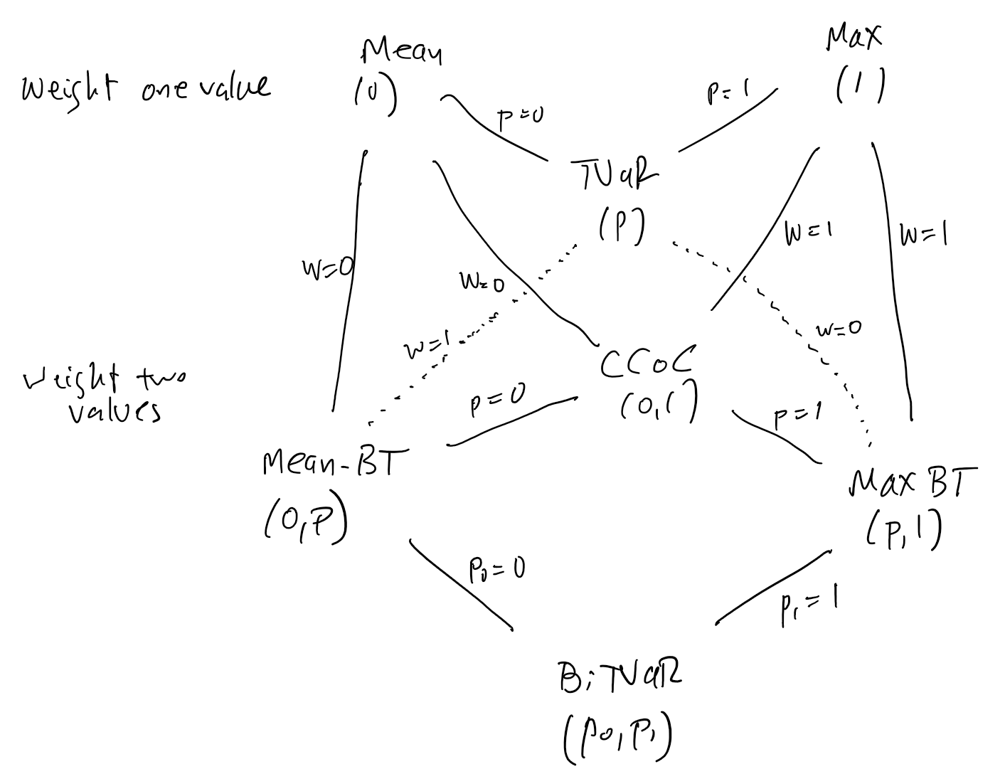
By REF all distortions can be written as a weighted average of TVaRs. The mean (max) distortion is the TVaR at $p=0$ ($p=1$) are special cases of TVaRs. A BiTVaR is a weighted average of two TVaRs. The general form of a BiTVaR is \[ g(s) = w\left(\displaystyle\frac{s}{1-p_1}\right) + (1-w)\left(\displaystyle\frac{s}{1-p_0}\right) \] for $0\le p_0<p_1\le 1$ and $0\le w\le 1$. The weight is applied to the larger $p$ value. Allowing for special and degenerate cases, there are seven types of BiTVaR:

The mean $g(s)=s$ weights $p=0$.
The maximum $g(0)=0$, $g(s)=1$ for $s>0$ weights $p=1$.
A (pure) TVaR $g(s)=\displaystyle\frac{s}{1-p}\wedge 1$ weights $p\in(0,1)$.
The constant cost of capital (CCoC) $g(s)=d + vs$, $d,v\in(0,1)$ and $d+v=1$, weights $0$ and $1$; it is a weighted average of mean and max.
A mean-BiTVaR weights $p_0=0$ and $p_1\in(0,1)$.
A max-BiTVaR weights $p_0\in(0,1)$ and $p_1=1$.
A (pure) BiTVaR weights $p_0<p_1$ with $p_0,p_1\in(0,1)$.

Figure 2.1 lays out the relationships between these seven types.

definitions and examples
characterize distortions achieving a given price
diagram from BTE of types

Note there is an asymmetry between mean and max behavior. Weight max means not continuous at $0$. Weight min means $g’(1)>0$. $g$ can only be discontinuous at $s=0$.

2.6.10 Calibrating distortions to market pricing

Newton Raphson trick

2.6.11 Risks with a given price from a given distortion

Point being?

2.6.12 Bid and ask prices with an SRM

definitions and examples

The bid price $B(X)=-A(-X)$, since, having written $-X$ on the ask, selling $X$ on the bid yields the zero portfolio which has zero value and so $A(-X) + B(X)=0$ by no arbitrage. It follows that \[ B(X)=\inf_{\mathsf Q\in \mathcal D} \mathsf E_\mathsf{Q}[X]. \] These facts are explained in Follmer et al. (2016), Mildenhall and Major (2022).

Comonotonic additive risk measures are normalized because $\rho(0)=\rho(0+0) = \rho(0) + \rho(0)$. SRMs are cash (translation) invariant, meaning $\rho(x+X) = x + \rho(X)$ for constant $x$. Applied to $X=0$ and using the normalized property, this shows that cash is riskless: $\rho(x)=x$.

2.6.13 NA P and M

Natural allocation and calcuation formulae
$\kappa$
Equally weighted simulations $X_i$ by unit $i$
Probability adjustment $Z$
- A set of non-negative factors that sum to 1, meaning $\mathsf E[Z]=1$
- Give the risk-adjusted probability of each scenario
$\mathsf E[XZ]$, the average of $X \times Z$, equals the risk-adjusted expected value of $X$
$Z$ is calibrated so that $M:=\mathsf E[XZ]-\mathsf E[X]$ equals the desired underwriting margin
$\mathsf E[X_iZ]$ is the risk-adjusted expected value of unit $i$ and $M_i:=\mathsf E[XZ]-\mathsf E[X]$ its allocated margin
$M=\sum_i M_i$ “adds-up”
Hurdle $=1-M_i/P_i$ is computed from the plan premium by unit

2.6.14 NA Q and average cost Q

2.6.15 Covariance interpretation of NA P

$\mathsf{Cov}(X_i, Z)=\mathsf E[X_iZ]-\mathsf E[X_i]\mathsf E[Z]=\mathsf E[X_iZ]-\mathsf E[X_i]$ because $Z$ sums to 1
Hence we can write the premium $\mathsf E[X_iZ]=\mathsf E[X_i] + \mathsf{Cov}(X_i, Z)$ showing the covariance equals the risk margin
Covariance is hard to interpret because it depends on scale
Correlation coefficient is a scaled version of covariance, analogous to CV
$\mathsf{corr}(X_i, Z):=\dfrac{\mathsf{Cov}(X_i,Z)}{\sigma_{X_i}\sigma_Z}$
Expressed using correlation coefficient, premium equals \[\mathsf E[X_i] + \mathsf{corr}(X_i, Z)\sigma_{X_i}\sigma_Z = \mathsf E[X] + \mathsf{corr}(X_i, Z)\mathsf E[X_i] \mathsf{cv}(X_i)\sigma_Z\] where the last term is the CV of $X_i$. This equation shows the risk load has three components:
1. Size: the expected losses of the unit, $\mathsf E[X_i]$
2. Volatility: the coefficient of variation of the unit, $\mathsf{cv}(X_i)$
3. Correlation: of losses with $Z$
$\mathsf{corr}(X_i, Z)$ is a measure of systematic risk for the unit within the total book; it improves over $\mathsf{corr}(X_i, X)$ by tempering extreme outcomes
$\sigma_Z$ is a little less than 1 in most cases and is a constant determined by $Z$

2.6.16 Strassen and Second-Order Stochastic Dominance

Stoyan p. 25

For $X$ and $Y$ with finite means, tfae

$X\le_{cx} Y$
there exists $X'$, $Y'$ with the same distributions as $X$, $Y$, such that $\mathsf E[Y'\mid X']=X'$ a.s., and in addition the conditional law $Y'\mid X'$ is stochastically increasing in $x$

Recall $X \le_{cx} Y$ means $\mathsf E[f(X)]\le\mathsf E[f(Y)]$ for all convex $f$. Since $f(x)=\pm x$ are both convex this implies $\mathsf E[X] = \mathsf E[Y]$.

Get the usual magic that we can do the MPS that walk from one distribution to the other, Machina and Pratt (1997).

2.6.17 OTHER OLD MATERIAL BROUGHT FORWARDS

2.6.18 Optimizations

Maximize profit subject to a capital constraint

Profit rates $\pi_i$ given by market conditions
Volumes $v_i$ selected by company
Capital function $\alpha$ specified by regulator or rating agency
Optimization: maximize dollar profit subject to capital constraint: $\max v\pi$ over $v$ subject to $\alpha(v) \le K$
Solution using Lagrangian multipliers satisfies $\pi = \lambda \displaystyle\frac{\partial \alpha}{\partial v }$, i.e., $\nabla \alpha\propto \pi$
No guarantee that optimal solution hits cost of capital constraint
- Add cost of capital $v\pi = \iota K$ solves for $\lambda$ and hence $\nabla \alpha$
- Solution may not exist (looking for point on surface with given marginal slopes)
Need differentiable capital function
- VaR does not have stable derivative (coVaR)
- TVaR does have stable derivative (coTVaR)
- SP-like premium and reserve risks are linear and easy to differentiate
Analysis ignores default implications

Marginal Cost of Capital

Cost of risk equals $\rho_\alpha(X):=\rho(X\wedge \alpha(X))$ where $\rho$ is the SRM pricing capital, $\alpha$ is the regulator/rating agency capital function, and $\wedge$ means minimum
$\rho(X\wedge \alpha(X)) = \displaystyle\int_0^{\alpha(X)} g(S(x))dx$
$X=X(v)$ is a function of volume in some way; if linear (homogeneous) then know derivatives of survival and quantile functions (inverses) and TVaR function
Marginal cost of capital equals \[\frac{\partial \rho_\alpha}{\partial v} = \displaystyle\int_0^{\alpha(X)} \frac{\partial }{\partial v} g(S_v(x))dx + g(S(\alpha)) \frac{\partial \alpha}{\partial v}\]
$\dfrac{\partial }{\partial v} g(S_v(x)) = g'(S(x))\dfrac{\partial S}{\partial v}$, with the latter partial depending on the stochastic model
For a homogeneous model, $\dfrac{\partial S}{\partial v}=\mathsf E[X_i \mid X]$

Case of TVaR Capital Measure $\alpha$

For $\alpha=\mathsf{TVaR}$ we get \[\frac{\partial \rho_\alpha}{\partial v} = \displaystyle\int_0^{\alpha(X)} g'S(x))\frac{\partial S}{\partial v} dx + g(S(\alpha)) \mathsf E[X_i \mid X > \mathsf{VaR}(X)]\] which for a homogeneous portfolio gives \[\frac{\partial \rho_\alpha}{\partial v} = \mathsf E_g[X \mid X\le \mathsf{TVaR}(X)] (1-g(S(\alpha)) + \mathsf E[X_i \mid X > \mathsf{VaR}(X)]g(S(\alpha))\]
- The first term is the “cost of volatility” the impact of the change in the shape of the distribution across all loss levels up to $\alpha$
- $\mathsf E_g$ is the risk adjusted expected value using distorted probabilities
- The second term is the cost of additional capital caused by marginal growth
The blending depends on the properties of $g$

Reduction to marginal capital

In order to reduce to marginal capital, must have $g'(S(x)))=0$ for $x<\alpha$ which implies $g(s)=1$ for $s > \Pr(X > \alpha)$
Lowest cost option is TVaR, reducing to coTVaR, since $g(S(\alpha))=1$
Other, higher cost, options possible

2.7 Life Actuarial

2.7.1 Time periods in discounting tabulations, why time starts at $t=0$

2.7.2 Dicounting, $v+d=1$, $v=1/(1+d)$, $d=1-v$

2.7.3 Equivalence principle premium

Equivalence principle premium (Dickson et al. 2015, Ch 6)

2.7.4 Profit signature

2.7.5 PVI / PVP

2.8 Basic Premium Calculation Principles

Adding expense and profit allowances

2.8.1 Expense loadings

Fixed and variable expenses
Profit on commission (Fl HO), etc.
All variable, expense on profit
Variable, no expense on profit
Fixed and variable
Pay attention to the precise problem solved by each approach: what is the question each pricing framework answers? For example:
- $L / (1-e-\pi)$
- $(L+F)/(1-v-\pi)$
- $L/(1-\pi)/(1-v)$
- $PV(L) / (1-e-\pi)$

2.8.2 Basic premium calculation formulae

2.8.3 Premium from the top down

Top-down estimation and calibration of cost of underwriting risk (PB valuation, risk, investment return and risk)

2.8.4 Regulatory approaches

Solvency 2 cost of capital model (~~allocated~~ stand-alone capital x cost = risk adjustment)

2.9 Understanding Diversification

JRI Albrecht paper and RMIR why buy insurance papers.

2.9.1 Capital requirements and the impact of default

We operate with bounded random variables and assume capital sufficient to eliminate default. The actuarial pricing literature expends a significant focus on default risk (Ibragimov et al. 2010; Myers and Read Jr. 2001; Sherris 2006). However, when using an SRM prices rule, all of the interesting pricing phenomena¹ already appear in the no-default case. In practice, default has a very small probability and hence a de minimus impact on pricing. The case with default, where assets $a<\max(X)$, can be reduced to the no default case by replacing $X$ with $X\wedge a$ and each $X_i$ with its associated recovery under the relevant default rule. See Mildenhall and Major (2022) Section 14.3.4 for further discussion.

The insurance pricing literature usually pays very close attention to default. However, in a well-functioning market, default should have a de minimus impact on pricing because it is a rare event. This intuition is confirmed by looking at examples. It is instructive to consider how the shape of risk impacts price in the absence of default because such an analysis should still reveal interesting properties; see the analysis in Mildenhall and Major (2022) Section 14.3.4. With these facts in mind, we consider bounded $X$ and assume the insurer holds sufficient capital to pay all claims, i.e., there is no chance of default.

Allowing the possibility of default adds greatly to the model’s complication without revealing any interesting new behaviors. The complications include the level of confidence required at interim evaluations. Specifically, the model must address how much capital is necessary and the degree of certainty needed to ensure that one can purchase the policy for the subsequent period. These considerations are beyond the current scope and will be explored in further detail in subsequent analyses.

If the insurer only holds assets $a$ and is subject to limited liability and pays according to equal priority (Mildenhall and Major 2022, p. 8.2 and 12.3) there is a difference between the promised indemnity $X$ and the amount actually paid $X\wedge a:=\min(X, a)$. The ask price becomes $A(X\wedge a)$, see also the discussion in Albrecher et al. (2022). The additional wrinkles introduced by default are discussed in REF.

2.9.2 Why do riskier risks pay a higher margin?

transfer effects of default;
Efron risks;
non-Efron risks;
wild risks;
range of NA vs. stand-alone;
converting a risk to stand-alone pricing

Pricing vectors must be comonotonic with the total insurance outcome. I have a short paper planned on diversification that helps explain this. Here’s the short version. Insurers issue two types of securities to raise assets: insurance policies and equity/debt instruments. Policies pay more in bad states (to the insurer) and equity pays more in good states (thinking of a one period insurer that dividends its residual value, like a Lloyd’s syndicate at close). Policies are written at the insurer’s ask price. Equity is sold at the investor’s bid price. In aggregate the insurer collects a bid ask spread from insureds and pays it to investors, performing some pooling function along the way. An individual policy can be decomposed into a part comonotonic with total losses, that is priced the same as a stand-alone policy, and an offsetting counter-monotonic part that is priced like equity. Most of the time, the latter is zero, but sometimes it is not. The classic example is “diversifying cat”, which actually acts partially like financing. That’s why it is sold cheaper. (email to Morton Lane)

2.9.3 Transfer effects of default

2.9.4 Efron risks, non-Efron risks, and wild risks

2.9.5 Range of NA vs. stand-alone

2.9.6 Pricing as though SA

2.9.7 Four examples

constant and risky illustrates expected loss transfers.
Log concave illustrates pulling diversification benefit only.
Cat non-cat, ideally done with finite support, distributions, illustrates, pooling and ordering diversification.
Awkward example illustrates just ordering diversification.

Loss - action of Eq priority. X is all that matters. Risk prefs don’t. Alters exp loss. Cross subsidies.

Premium: X to projection of X pooling

Dependencies of projections. Simple examples. General case. U and D decomposition

Pooling paper

Bring X or it’s projection SA X ge SA projection that gives range info

If projections are comon w total: done. No further credit. Discuss when: Efron, iid, CP w same severity etc.

But not always. Samples w unique values there is no pooling benefit of this kind. Example showing still decent credit?

What when not comon? What’s going on?

Split risk into financing and insurance parts (diff of two increasing functions (how when multiple local max mins)) one priced on bid one on ask gives the NA price. What are the distributions of the incre and decr parts?

Examples

Simple single turning point
Complex multiple
Awkward

Questions

Positive / negative margin compared to promised indemnity
Positive / negative margin compared to actual indemnity (c.f. Albrecher et al. (2022))

2.10 Layering and Allocating Capital

2.10.1 Allocating capital and insurer management

Allocating capital presents the modeler with a problem. On the one hand, allocating capital does not make sense because all capital supports all risks and, it is not observable as is not booked anywhere. On the other, allocation terminology is embedded in management mindset and talk of “allocating capital” is common. Venter, Mildenhall and Major (2022), and others suggest allocating the cost of capital rather than capital, but the cost of a block of capital depends on the risk load put upon it, and the cost of equity is nebulous whereas capital structure is evident from the balance sheet.

Level	Capital	Margin
Corporation	On balance sheet	Target hard to determine
Unit	Possibly disclosed	Targeted by corporate
Account	Never booked	Set by market Estimated by actuaries

Thus, the amount capital is known at the corporate level and not at the account level, whereas its cost is hard to estimate at the corporate level but easier at the account level. For the CEO it is more natural to think about allocating (known) capital than (unknown) total margin; for the line-underwriter it is more natural to incorporate a margin into quoted premium or derive it from market rates than think about account-level capital.

Sometimes talk about allocation is inescapable, and so we need a sensible approach and guard rails around its use. Mildenhall and Major (2022) section 14.3.8 describes the natural allocation of capital (NAQ), a theoretically sound method, consistent with spectral risk measure pricing. However, NAQ is hard to interpret, because it earns a risk-adjusted (variable) profit: a large allocation does not necessarily equate to a high margin. The NAQ can also be negative and associated with a negative margin—though that is generally a sign of other issues!

In a limited liability, equal priority model losses by unit are contractually determined. The spectral methodology then determines a consistent premium using risk-adjusted probabilities and hence a margin by unit, all as functions of assets. These determinations are all additive and identify total capital via the funding equation $\bar Q(a)=a - \bar P(a)$². The natural allocation of $\bar Q$ to unit $i$ uses the fact that a law invariant risk measure has a constant return equal to $(g(s)-s) / (1-g(s))$ in the infinitesimal layer with probability $s$ of loss for all units, resulting in the allocation \[ \begin{aligned} \bar Q_i(a) &= \int_0^a \frac{\text{allocated margin in layer}}{\text{layer return}} \\ &\phantom{M} \\ &= \int_0^a \frac{\text{allocated margin in layer}}{\text{layer margin}} \times \text{layer capital} \\ &\phantom{M} \\ &= \int_0^a \frac{\beta_i(x)gS(x) - \alpha_i(x)S(x)}{gS(x)) - S(x)} \times (1 - g(S(x)))\, dx \\ &= \int_0^a \frac{M_i(x)}{M(x)} \times Q(x)\, dx \\ \end{aligned} \] since $M_i(x) = \beta_i(x)gS(x) - \alpha_i(x)S(x)$ is the margin in the layer “at $x$” (which attaches with probability $S(x)$). This method allocates assets within each layer in proportion to margin.

A alternative approach is to assume that the cost of capital is constant within each tranche of capital, as opposed to infinitesimal layer. A tranche could be a layer (subordinated, senior, etc.) of debt, or the remaining equity tranche, or in the case of all-equity financing it is all capital. This assumption is reasonable because all agents are equal within a tranche. The layer is priced at a consensus rate acceptable to all agents who buy it, but likely not exactly equal to their reservation prices. Thus, unlike the theoretic model, the pricing is an approximation. It can be regarded as a CCoC distortion approximation to the true (but unknown) underlying distortion derived by the distortions of the participating agents.

When there is a single tranche of capital (all-equity financing), the constant average-cost of capital allocation is derived by dividing each unit’s natural allocation margin by the tranche’s average return. For a single tranche $[0, a]$ this equals \[ \begin{aligned} \bar Q^c_i(a) &= \frac{\text{allocated tranche margin}}{\text{tranche average return}} \\ &\phantom{M} \\ &= \frac{\text{allocated tranche margin}}{\text{tranche margin}} \times \text{tranche capital} \\ &\phantom{M} \\ &= \frac{\int_0^a \beta_i(x)gS(x) - \alpha_i(x)S(x)\,dx}{\int_0^a 1 - g(S(x))\,dx} \times \int_0^a 1 - g(S(x))\,dx \\ &= \frac{ \bar M_i(a) }{ \bar M(a) } \bar Q(a). \end{aligned} \] The last line reminds us this method is allocating assets in proportion to margin, except at the whole tranche level rather than at the infinitesimal layer level. For a tranche from $a_0$ to $a_1$ the integrals become $\int_{a_0}^{a_1}$ and margin $\bar M_i(a_1)-\bar M_i(a_0)$. Call this the constant cost of capital allocation, written Q_const in tables.

This section explores the difference between these two approaches. First, some general remarks. There are several confounding effects that make it difficult to target returns by unit. Generally, for a given distortion and capital standard, an all-equity tranche will have a lower return for a more skewed risk because such a risk uses more, cheaper tail capital. The risk has a high premium margin because the lower cost of capital is offset by lower leverage. However, when thick and thin tailed risks are combined in a portfolio, there are inter-risk transfers, whereby a thick tailed line benefits from pooling with a thin tailed one in a poorly capitalized pool. (In insolvent states the thick tailed line has a larger loss and captures a greater share of the available assets under equal priority.) As a result, the thick tailed line needs to pay a higher margin, resulting in a payment to the thin tailed line that makes pooling attractive, see the plot of cumulative margin in the right-hand plot of Figure 3.1. In this case, the stand-alone intuition can fail, and the thick tailed line can have a higher cost of capital. These effects are more pronounced for poorly capitalized pools. We turn now to an example illustrating these ideas.

Acerbi, C. (2002). Spectral measures of risk: A coherent representation of subjective risk aversion. Journal of Banking & Finance, 26(7), 1505–1518. https://doi.org/10.1016/S0378-4266(02)00281-9

Albrecher, H., Eisele, K. T., Steffensen, M., & Wüthrich, M. V. (2022). On the cost-of-capital rate under incomplete market valuation. Journal of Risk and Insurance, 89(4), 1139–1158. https://doi.org/10.1111/jori.12406

Bielecki, T. R., Cialenco, I., & Liu, H. (2024). Time consistency of dynamic risk measures and dynamic performance measures generated by distortion functions. Stochastic Models. https://doi.org/10.1080/15326349.2024.2353045

Caramagno, N., Mamane, D., & Neilson, L. (2021). An Introduction to IFRS 17 for P&C Actuaries (pp. 1–25). Casualty Actuarial Society. https://www.ifrs.org/issued-standards/list-of-standards/ifrs-17-insurance-contracts/

Chang, J. T., & Pollard, D. (1997). Conditioning as disintegration. Statistica Neerlandica, 51(3), 287–317. https://doi.org/10.1111/1467-9574.00056

Cummins, J. D. (1990). Multi-Period Discounted Cash Flow Rate-making Models in Property-Liability Insurance. Journal of Risk and Insurance, 57(1), 79–109.

Dickson, D. C. M., Hardy, M. R., & Waters, H. R. (2015). Actuarial Mathematics for Life Contingent Risks (Vol. 1). Cambridge University Press. https://doi.org/10.1017/CBO9781107415324.004

Follmer, H., Schied, A., Föllmer, H., & Schied, A. (2016). Stochastic Finance: An Introduction in Discrete Time (Fourth.). Berlin, Boston: Walter de Gruyter. https://doi.org/10.1017/CBO9781107415324.004

Ibragimov, R., Jaffee, D., & Walden, J. (2010). Pricing and Capital Allocation for Multiline Insurance Firms. Journal of Risk and Insurance, 77(3), 551–578. https://doi.org/10.1111/j.1539-6975.2010.01353.x

International Accounting Standards Board. (2017). IFRS 17 - Insurance Contracts. https://doi.org/10.4324/9781315099842-7

Kusuoka, S. (2001). On law invariant coherent risk measures. Advances in Mathematical Economics, 3, 83–95. http://link.springer.com/chapter/10.1007/978-4-431-67891-5_4

Machina, M. J., & Pratt, J. W. (1997). Increasing Risk: Some Direct Constructions. Journal of Risk and Uncertainty, 14(2), 103–127. https://doi.org/10.1023/A:1007719626543

McClenahan, C. L. (1999). Insurance Profitability. Actuarial Considerations Regarding Risk and Return, 113–124.

Mildenhall, S. J., & Major, J. A. (2022). Pricing insurance risk: Theory and practice. John Wiley & Sons, Inc.

Myers, S. C., & Read Jr., J. A. (2001). Capital allocation for insurance companies. Journal of Risk and Insurance, 68(4), 545–580. http://www.jstor.org/stable/2691539

Pollard, D. (2002). A user’s guide to measure theoretic probability. Cambridge University Press.

Robbin, I. (2007). IRR, ROE, and PVI/PVE. Casualty Actuarial Society Forum, Winter, 189–256.

Sherris, M. (2006). Solvency, capital allocation, and fair rate of return in insurance. Journal of Risk and Insurance, 73(1), 71–96. http://onlinelibrary.wiley.com/doi/10.1111/j.1365-2966.2006.00166.x/full

Svindland, G. (2010). Continuity properties of law-invariant (quasi-)convex risk functions on $L^\infty$. Mathematics and Financial Economics, 3(1), 39–43. https://doi.org/10.1007/s11579-010-0026-x

Van Slyke, O. E. (1999). Actuarial Considerations Regarding Risk and Return in Property-Casualty Insurance Pricing (p. 179). Arlington, VA: Casualty Actuarial Society.

Wang, S. S. (2000). A class of distorion operators for pricing financial and insurance risks. Journal of Risk and Insurance, 67(1), 15–36.

The “interesting phenomena” are
- Sub-additive pricing and positive bid-ask spread
- Margin for non-diversifiable risk
They are caused by credit sensitive customers and costly capital (Mildenhall and Major 2022, sec. 8.2.5).↩︎
The bar is Mildenhall and Major (2022) notation for the cumulative amount up to asset level $a$.↩︎